Conditional Slopes in Interaction Models

The Slope of X as a Function of Z

In the previous lesson, we saw that for a model with a continuous predictor (X) and a binary moderator (Z), the slope of X was ${\beta }_1$ for the reference group (Z=0) and $({\beta }_1+{\beta }_3)$ for the other group (Z=1).

Now, what if the moderator Z is also a continuous variable, like age or experience_years? The model equation remains the same:
$\hat{Y}={\beta }_0+{\beta }_{1}X+{\beta }_{2}Z+{\beta }_3(X\cdot Z)$

The key insight is that the effect of X on Y is no longer a single number; it is now a function of Z. We can see this by rearranging the terms of the equation:
$\hat{Y}=({\beta }_0+{\beta }_{2}Z)+({\beta }_1+{\beta }_{3}Z)X$

Look closely at the term in the second parenthesis. This is the coefficient of X.

• The slope of X is $({\beta }_1+{\beta }_{3}Z)$.

This means for every one-unit increase in X, Y is predicted to change by $({\beta }_1+{\beta }_{3}Z)$. The slope itself depends on the value of Z. The following video provides an excellent conceptual recap of this idea.

Spotlight Analysis: Calculating Slopes for a Continuous Moderator

Since Z is continuous, it can take on infinitely many values. We can't calculate the slope of X for every single one. Instead, for exam purposes, you will use a standard method called spotlight analysis. This involves calculating the slope of X at a few representative values of the moderator Z.

The standard convention is to choose three values:

1. Average level of Z: The mean of Z, $\bar{Z}$.
2. High level of Z: One standard deviation above the mean, $\bar{Z}+\text{SD}(Z)$.
3. Low level of Z: One standard deviation below the mean, $\bar{Z}-\text{SD}(Z)$.

You then plug these three values into your slope equation, $({\beta }_1+{\beta }_{3}Z)$, to get three different "simple slopes" for X.

The following reading demonstrates this calculation with a clear, step-by-step example.

After calculating these slopes, you can visualize them as three distinct regression lines, showing how the relationship between Y and X changes as Z changes.

How to Interpret Simple Slopes Output

On an exam, you might be given an output table that has already calculated these simple slopes for you. Your task is to interpret it correctly.

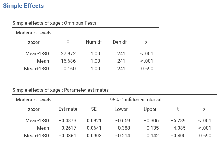
What to look for and how to interpret it:

1. Moderator Levels: The first column shows the specific values of the moderator (zexer) used for the calculation (Mean-1SD, Mean, Mean+1SD).
2. Estimate: This is the key value. It is the calculated slope of the predictor (xage) at that specific level of the moderator.
   • Exam-style sentence: "When zexer is one standard deviation below its mean, the slope of xage is -0.4873. This means for a one-unit increase in xage, the response is predicted to decrease by 0.4873, at this specific level of zexer."
3. p-value: This tells you whether that specific simple slope is statistically significant (i.e., different from zero).
   • Exam-style sentence: "The relationship between xage and the response is statistically significant when zexer is at its mean (p < .001) and one standard deviation below its mean (p < .001), but it is not significant when zexer is one standard deviation above its mean (p = 0.690)."

This analysis is far more nuanced and precise than just looking at the main interaction coefficient. It tells you where the interaction is happening.

For those interested in the full manual derivation of these simple slopes, the following resource provides an excellent, though optional, walkthrough.

Practice Drill

You are analyzing housing prices and fit the following interaction model. The response is price (in thousands of dollars), and the predictors are size (in square feet) and age (in years).

Model Output:

Coefficients:
                 Estimate Std. Error t value Pr(>|t|)
(Intercept)      150.000    10.000   15.00   <2e-16 ***
size               0.250     0.050    5.00    <2e-16 ***
age               -2.000     0.500   -4.00    0.0001 ***
size:age          -0.005     0.001   -5.00    <2e-16 ***

You are also given that for the variable age:

• Mean = 20 years
• Standard Deviation = 10 years

Your Task:

1. Write down the general equation for the slope of size.
2. Calculate the simple slope of size for a house of average age (20 years). Interpret this slope.
3. Calculate the simple slope of size for a new house (one SD below the mean age).
4. Calculate the simple slope of size for an old house (one SD above the mean age).
5. In one sentence, what does this interaction tell you about the effect of house size on price?

Conclusion

You have now learned how to probe an interaction term to find the simple slopes, which is a powerful and precise method of interpretation. This moves beyond simply stating "the effect depends" to explaining how it depends.

Key Takeaways:

• In a model with an interaction term $X\cdot Z$, the slope of X is given by the equation $({\beta }_1+{\beta }_{3}Z)$.
• To interpret a continuous-by-continuous interaction, you calculate the slope of X at specific, representative values of Z.
• The standard approach ("spotlight analysis") is to use the mean of Z, one standard deviation above the mean, and one standard deviation below the mean.
• Exam outputs may provide these "simple effects" directly, and you must be able to interpret the slope (Estimate) and its significance (p-value) for each level of the moderator.

This lesson completes our deep dive into interaction models. In our final lesson of this module, we will explore another essential technique for improving regression models: log transformations. We will see how transforming a variable can help fix violations of key assumptions like linearity and homoscedasticity.