Detecting Multicollinearity with VIF

Welcome to the first lesson in our new module on advanced diagnostics. Having just learned how to use transformations to fix violations of model assumptions, we now turn our attention to a different kind of issue: problems that arise from the relationships between your predictor variables.

Today's lesson addresses multicollinearity. This occurs when your predictor variables are not independent but are instead correlated with each other. This is a common and subtle problem that can severely undermine your ability to interpret your model's results. We will focus on precisely what multicollinearity is, why it's a problem for your analysis, and, most importantly, how to use the Variance Inflation Factor (VIF) to detect and quantify it.

What is Multicollinearity?

In simple terms, multicollinearity means that two or more of your independent (predictor) variables are highly correlated. When this happens, they carry redundant information. The model struggles to disentangle their individual effects on the response variable.

Imagine you're building a model to predict house prices, and you include both "house size in square feet" and "number of bedrooms" as predictors. These two variables are likely to be highly correlated—larger houses tend to have more bedrooms. The model will find it difficult to determine how much a price increase is due to the extra square footage versus the additional bedroom, because they almost always change together.

This short video provides a clear, intuitive explanation of this exact problem.

Multicolinarity - An Easy and Clear Beginner’s Guide

This video from the channel numiqo gives a great beginner-friendly introduction to the concept of multicollinearity using the house price example.

Watch the first two minutes, from the beginning to the introduction. Focus on the core idea: when predictors overlap, the model can't reliably determine their individual coefficients.

The Consequences of Multicollinearity

For your exam, you must be able to state precisely why multicollinearity is a problem. While it often doesn't harm the overall predictive accuracy of the model, it severely compromises the interpretability of the individual coefficients.

The StatTrek article on multicollinearity provides a concise summary of the key issues.

Multicollinearity and Regression

This article clearly lays out the practical consequences of multicollinearity.

Read the section titled The Multicollinearity Problem. Pay close attention to the two main consequences it highlights.

As you just read, the two primary consequences of high multicollinearity are:

Unreliable Coefficient Estimates: The estimated coefficients for the correlated predictors can become very unstable. A small change in your data (like adding or removing a few observations) could cause the signs of the coefficients to flip or their magnitudes to change dramatically. This makes them untrustworthy.
Inflated Standard Errors: The standard errors of the coefficients for collinear variables increase. This leads to wider confidence intervals and smaller t-statistics. As a result, a predictor that is actually important might appear statistically insignificant (i.e., have a large p-value).

Common Exam Trap: A question might show a model with a high R-squared (good overall fit) but with several insignificant predictors. This is a classic symptom of multicollinearity. Remember: multicollinearity affects the interpretation of individual predictors, not necessarily the overall predictive power of the model.

Detecting Multicollinearity: The Variance Inflation Factor (VIF)

The best way to detect multicollinearity is by calculating the Variance Inflation Factor (VIF) for each predictor in your model. The VIF measures how much the variance of an estimated regression coefficient is "inflated" because of its correlation with other predictors.

The intuition behind the VIF calculation is clever. For each predictor $X_{j}$ , you run an "auxiliary" regression where $X_{j}$ is treated as the outcome, predicted by all the other independent variables in your model.

From this auxiliary regression, you get an $R^{2}$ value, which we'll call $R_{j}^{2}$ . This $R_{j}^{2}$ tells you how well predictor $X_{j}$ is explained by a linear combination of the other predictors. The VIF for that predictor is then calculated using a simple formula.

The following video explains this process clearly.

Variance Inflation Factors: testing for multicollinearity

This video by Ben Lambert explains the logic behind VIF by walking through the concept of auxiliary regressions.

Watch the segment from construction of VIF. The key takeaway is understanding that VIF is derived from running a separate regression for each predictor to see how well it's explained by the others.

As the video explained, the formula is:

V I F_{j} = \frac{1}{1 - R _{j}^{2}}

Think about what this means:

If $R_{j}^{2} = 0$ , the predictor $X_{j}$ is completely uncorrelated with the others. The VIF is $\frac{1}{1 - 0} = 1$ . This is the baseline (no inflation).
If $R_{j}^{2}$ is high (e.g., 0.9), it means $X_{j}$ is highly redundant. The VIF is $\frac{1}{1 - 0.9} = 10$ . This indicates a serious problem. The variance of the coefficient for $X_{j}$ is 10 times larger than it would be if there were no multicollinearity.

Interpreting VIF: The Exam-Ready Rules

Most statistical software, including R, will calculate VIFs for you. You will typically see it as an additional column in your regression output or as a separate table or plot. Your job is to interpret these values.

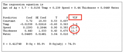
A typical regression output from statistical software like Minitab, showing a VIF column. Here, 'Speed' and 'Thickness' have problematically high VIF values.

A bar chart is another common way to visualize VIFs. The dashed red line often represents a threshold for concern.

For your exam, use these rules of thumb to interpret the VIF values. The DataCamp tutorial provides a great summary.

Variance Inflation Factor: How to Detect Multicollinearity

This section gives you clear, tiered rules for interpreting VIF values.

Read the section titled Interpretation of VIF Values. Commit these thresholds to memory.

Here is a summary of the interpretation guidelines for your exam answers:

VIF = 1: No multicollinearity. The predictor is not correlated with others.
VIF between 1 and 5: Moderate multicollinearity. This is generally considered acceptable and not a cause for concern.
VIF > 5: High multicollinearity. This is a potential red flag.
VIF > 10: Serious multicollinearity. Your syllabus specifically highlights this threshold. A VIF above 10 indicates that the coefficient estimates are likely unstable and their p-values are unreliable. This requires action.

Practice Drill

You are given the following R output for a model predicting employee Salary (in thousands of dollars) based on YearsExperience, Age, and TrainingHours.

Coefficients:
                Estimate Std. Error t value Pr(>|t|)   VIF
(Intercept)      25.102      5.210   4.818 1.45e-06 ***
YearsExperience   2.981      0.852   3.499 0.000512 ***  12.5
Age               1.520      0.799   1.902 0.057890 .    11.8
TrainingHours     0.155      0.032   4.843 1.29e-06 ***   1.2

Residual standard error: 5.12 on 296 degrees of freedom
Multiple R-squared:  0.921,	Adjusted R-squared:  0.920
F-statistic: 1152 on 3 and 296 DF,  p-value: < 2.2e-16

Your Task:
Provide a 2-3 line exam-style answer for each of the following questions:

Identify which variables, if any, suffer from problematic multicollinearity. Justify your answer using their VIF values.
Explain the likely consequence of this multicollinearity on the Age coefficient's p-value.

Solution

The variables YearsExperience and Age suffer from serious multicollinearity. Their VIF values of 12.5 and 11.8 are both well above the common threshold of 10, indicating a strong linear relationship between them.
The high multicollinearity has likely inflated the standard error of the Age coefficient. This makes the coefficient appear statistically insignificant (p-value = 0.058), even though Age might be an important predictor of salary. The model cannot confidently separate the effect of Age from the effect of YearsExperience.

Conclusion

You now have a complete framework for diagnosing multicollinearity, one of the key challenges in multiple regression. This is an essential skill for building reliable and interpretable models.

Key Takeaways:

Definition: Multicollinearity is a high correlation between two or more predictor variables.
Consequences: It causes unstable coefficient estimates and inflated standard errors, making it difficult to assess the significance of individual predictors.
Detection: The primary tool is the Variance Inflation Factor (VIF).
Interpretation: A VIF value greater than 10 indicates a serious multicollinearity problem that needs to be addressed.

This lesson concludes our introduction to multicollinearity. In the next lesson, we will continue our module on advanced diagnostics by examining another type of data issue: high-leverage and high-influence points, which are individual observations that can have an outsized impact on your entire model.