Introduction
In our last lesson, we focused on calculating the after-tax cash flows for a capital project, which are the essential inputs for our financial analysis. Now that we have these figures, we can begin to evaluate whether a project is worth pursuing.
This lesson introduces two of the simplest and most intuitive capital budgeting techniques: the payback period and the discounted payback period. The central question these methods ask is straightforward: "How long will it take to get our money back?" We will learn how to calculate both metrics and understand their strengths and weaknesses as decision-making tools. While they are often used as a preliminary screening method, mastering them is a key step before we move on to more comprehensive techniques like Net Present Value (NPV).
The Payback Period (PP)
The payback period is the length of time required for a project's cumulative net cash inflows to equal its initial investment. It's a measure of liquidity, indicating how quickly a project can return the initial capital outlay.
To calculate it, we track the cumulative cash flow year by year. Let's explore the method with a video.
This video from The Finance Storyteller provides a clear, conceptual introduction to the payback period and its calculation.
Please watch the following segments: First, understand the central question that the payback method answers. Next, follow the step-by-step calculation. The video demonstrates the cumulative cash flow approach, which is the standard method for projects with uneven cash flows.
As the video showed, the calculation involves two main steps:
- Sum the cash flows year by year until the cumulative total is no longer negative. The last full year before this happens is the "full years" part of our answer.
- Calculate the fraction of the next year needed to cover the remaining shortfall. The formula for the payback period is:
For a more detailed breakdown and another example, please review the following text.
Payback and discounted payback | Foundations in Accountancy
This article from ACCA Global provides a solid, exam-oriented explanation of the payback method.
Please read the section titled Payback. Focus on the definition and the first example, which uses a table to track cumulative cash flow. Then, review the calculation for the fractional year.
The decision rule for the payback period is simple:
- A company will typically set a maximum acceptable payback period (e.g., three years). If a project's payback period is less than this cutoff, it is accepted.
- When comparing two mutually exclusive projects, the one with the shorter payback period is generally preferred.
The Discounted Payback Period (DPP)
A significant weakness of the regular payback period is that it ignores the time value of money—it treats a dollar received in year 5 the same as a dollar received in year 1. Your work as a statistician has likely given you a strong intuition for weighting outcomes, and in finance, we weight future cash flows by discounting them.
The discounted payback period (DPP) corrects this flaw by using the present values of cash flows. It answers the question: "How long does it take for the cumulative discounted cash inflows to recover the initial investment?"
Because future cash flows are worth less in today's terms, the DPP will always be longer than the regular payback period for the same project.
Let's see how this is calculated.
The same video from The Finance Storyteller now explains the discounted payback method.
Please watch the following segments: First, understand the key difference between the regular and discounted payback methods. Next, watch the detailed explanation of how to calculate the present value of each cash flow using a given discount rate. The formula is PV = \frac{CF_t}{(1+r)^t}, where r is the discount rate and t is the year. Finally, see how these present values are used to find the discounted payback period using the cumulative discounted cash flow.
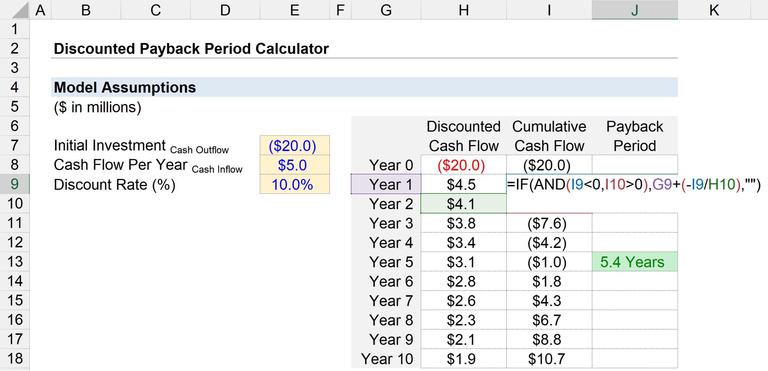
The process is almost identical to the regular payback calculation, but with one extra step at the beginning:
- Calculate the present value (PV) of each cash inflow.
- Calculate the cumulative discounted cash flow for each period.
- Use the same formula as before, but with the discounted values:
This calculation is clearly illustrated in the spreadsheet below.
A Worked Example
Let's solidify this with an example that combines everything.
A project has an initial investment of $100,000. The after-tax cash flows are projected as follows:
- Year 1: $30,000
- Year 2: $40,000
- Year 3: $50,000
- Year 4: $60,000
The company's discount rate is 12%. Let's calculate both payback periods.
1. Regular Payback Period (PP)
| Year | Cash Flow | Cumulative Cash Flow |
|---|---|---|
| 0 | ($100,000) | ($100,000) |
| 1 | $30,000 | ($70,000) |
| 2 | $40,000 | ($30,000) |
| 3 | $50,000 | $20,000 |
The payback occurs during Year 3.
- Full years = 2
- Unrecovered amount at start of Year 3 = $30,000
- Cash flow during Year 3 = $50,000
2. Discounted Payback Period (DPP)
First, we discount the cash flows at 12%.
| Year | Cash Flow | Discount Factor @12% | Discounted CF (PV) | Cumulative Discounted CF |
|---|---|---|---|---|
| 0 | ($100,000) | 1.000 | ($100,000) | ($100,000) |
| 1 | $30,000 | 0.893 | $26,790 | ($73,210) |
| 2 | $40,000 | 0.797 | $31,880 | ($41,330) |
| 3 | $50,000 | 0.712 | $35,600 | ($5,730) |
| 4 | $60,000 | 0.636 | $38,160 | $32,430 |
The discounted payback occurs during Year 4.
- Full years = 3
- Unrecovered PV at start of Year 4 = $5,730
- PV of cash flow during Year 4 = $38,160
As expected, the DPP is longer than the PP.
Usefulness and Limitations
While easy to calculate and understand, both payback methods have a critical flaw. Let's explore the pros and cons.
Payback and discounted payback | Foundations in Accountancy
This article concludes with a summary of the usefulness and drawbacks of these methods.
Read the short sections on Usefulness under both the Payback heading and the Discounted Payback heading. The key disadvantages listed for the regular payback period are also important to note.
The most significant disadvantage, which applies to both the regular and discounted payback methods, is that they ignore all cash flows that occur after the payback period.
Consider two projects, A and B, each costing $1,000.
- Project A pays back $1,000 in Year 1 and nothing thereafter.
- Project B pays back $1,000 in Year 2, and then $5,000 a year for the next 10 years.
Based on payback period alone, Project A is superior. However, Project B is clearly far more profitable. This is why payback is considered a measure of risk and liquidity, not profitability.
Conclusion
In this lesson, we have learned how to calculate and interpret the payback period and the discounted payback period. These methods provide a quick gauge of how long it takes for a project to return its initial investment.
Key Takeaways:
- The Payback Period (PP) measures the time to recover the initial investment using nominal cash flows. It is simple but ignores the time value of money.
- The Discounted Payback Period (DPP) corrects this by using cash flows discounted to their present value. It is a more financially sound measure than the simple PP.
- Both methods are calculated by tracking the cumulative cash flow (or cumulative discounted cash flow) until it turns positive.
- The primary advantages of these methods are their simplicity and their focus on liquidity and risk.
- The main disadvantage of both methods is that they completely ignore cash flows occurring after the payback period, meaning they are not reliable measures of a project's overall profitability.
Because of this major flaw, payback methods are best used as a secondary tool or for initial screening. In our next lesson, we will explore the Net Present Value (NPV), a superior investment appraisal technique that overcomes this limitation by considering all of a project's cash flows over its entire life.