Hello! Welcome to the final lesson of our course on database system internals.
In our previous lessons, we've explored various ways to optimize query performance, from materialized views that pre-compute results to column-oriented storage that accelerates analytical scans. These techniques generally require significant upfront design and tuning, often by a database administrator (DBA) who must anticipate the query workload.
Today, we'll explore a fascinating and more dynamic approach that challenges this traditional model. We'll examine what happens when the database system itself takes on the role of the tuner, building and refining indexes automatically as a direct consequence of processing queries.
This brings us to our final learning outcome: Describe the concept of adaptive indexing, where indexes are built incrementally during query processing. We will see how a system can learn from the queries it receives and physically reorganize data on the fly to accelerate future queries, without any upfront configuration.
The Bottleneck of Traditional Indexing
State-of-the-art database performance has long relied on having the right indexes. A B+ tree, for example, can turn a full table scan that takes minutes into a millisecond point lookup. The problem is, how do we know which indexes are the "right" ones?
The traditional approach is what we can call offline indexing:
- Analyze Workload: A DBA studies the queries the application is expected to run.
- Choose Indexes: Based on this analysis, the DBA decides which columns to index.
- Build Indexes: The system then spends a significant amount of time and resources—often hours for large tables—building these index structures. During this time, the system is either offline or under heavy load.
This model breaks down in modern data exploration scenarios. Imagine a scientist receiving a terabyte of new experimental data every day. The queries are exploratory by nature; the scientist doesn't know what they're looking for until they start looking. There is no pre-defined workload to analyze and no "idle time" to build indexes. By the time a traditional index is built, the workload may have already changed.
This is the core motivation for a new paradigm. What if we could eliminate the upfront tuning phase entirely?
Adaptive Indexing: Learning from Queries
Adaptive indexing flips the traditional model on its head. Instead of treating queries merely as questions to be answered, the system also treats them as hints about how the data should be physically organized. The index is not a static structure built beforehand; it is an emergent property that is built and refined incrementally, as a side-effect of query processing.
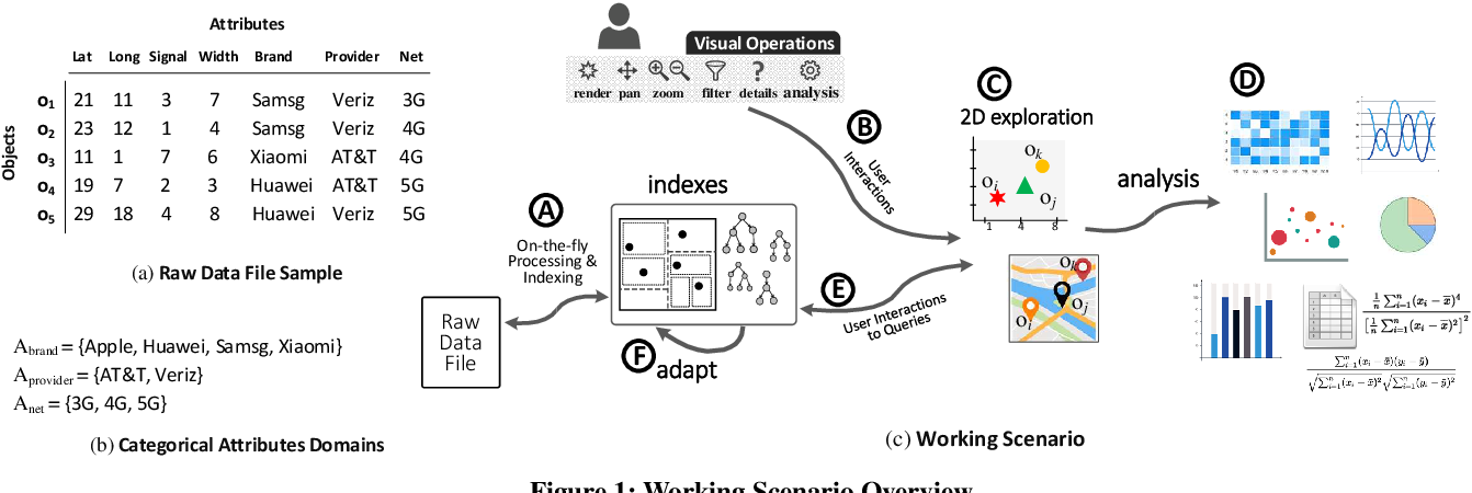
The foundational work in this area is a technique known as Database Cracking. Let's explore this concept in detail.
To understand the motivation and core idea, we'll read a few sections from 'Big Data Exploration' by Stratos Idreos (the creator of Harvard's CS165 course). This text perfectly frames the problem and introduces database cracking.
Please read the following three short sections: Start at the heading 'Adaptive Indexing' and read to the end of the subsection 'Big Data Indexing Problems'. This defines the problem with the traditional 'offline' approach. Continue with the subsection 'Database Cracking'. This introduces the concept of continuous, on-demand adaptive indexing. Finally, read the subsection 'Selection Cracking Example' to see a concrete illustration of how a query physically reorganizes a column.
As you just read, the central idea of cracking is to physically reorder a column based on a query's predicates. If the first query is SELECT ... WHERE A < 10, the system doesn't just find those records. As part of the query execution, it moves all values less than 10 to the beginning of the column and all values greater than or equal to 10 to the end.
The column is now "cracked" into two pieces. A subsequent query like SELECT ... WHERE A < 5 only needs to scan the first piece, while a query like SELECT ... WHERE A > 50 only needs to scan the second piece. With every query, the data becomes more organized, and future queries get faster.
The Architecture of a Cracking System
To make this concept concrete, let's look at the components needed to implement cracking, as detailed in the original paper.
The seminal 2007 paper, 'Database Cracking', lays out the architecture and algorithms. We'll read the section that describes the core data structures.
Please read Section 3, titled 'CRACKING' (it's about one page long). Focus on understanding the roles of the cracker column and the cracker index (AVL-tree). The figure in this section is particularly helpful.
Let's recap the key components from the paper:
- Cracker Column: When a column is first queried, a copy of it is created. This copy, the
cracker column, is where all the physical reorganization (cracking) happens. The original column is left untouched, preserving the original insertion order, which is useful for reconstructing full tuples later. - Cracker Index: A main-memory data structure, typically an AVL tree, that keeps track of the partitions. Each node in the tree stores a pivot value and the physical boundary of the piece it defines in the cracker column. When a query arrives, the system consults this index to find which piece(s) it needs to process and potentially crack further.
The Cracking Algorithms
So, how does the system perform this physical reorganization? The core operation is an in-place partitioning algorithm, which should be familiar to you from your background in algorithms (think of the partitioning step in Quicksort).
The original cracking paper defines two main algorithms for this.
Now let's examine the algorithms that perform the actual data movement. The same paper provides a clear description.
Please read Section 5, 'CRACKING ALGORITHMS'. Pay attention to the high-level goal of Algorithm 1 (CrackInTwo) and Algorithm 2 (CrackInThree). You don't need to trace the code line-by-line, but understand that they are cache-conscious, in-place partitioning algorithms that use the query's range predicate to define the pivot(s).
The key takeaway from the algorithms section is that cracking is not just a theoretical idea; it's implemented with efficient, low-level partitioning routines. These algorithms scan a piece of a column and swap elements so that all qualifying values end up in a contiguous block, creating new, smaller pieces. The pivot for the partition is not chosen randomly as in some quicksort variants, but is taken directly from the query predicate (e.g., 10 in the query A < 10).
Test your understanding!
Imagine a column that has just been cracked by the query WHERE val < 100. The cracker index now knows about two pieces: one for val < 100 and one for val >= 100.
Now, a new query arrives: WHERE val > 150.
Which piece(s) of the column does the system need to scan and crack? And what new pieces will be created?
Show answer
The system consults the cracker index and determines that the range val > 150 falls entirely within the second piece (val >= 100).
Therefore, it only needs to scan and crack that second piece. It will use a CrackInTwo algorithm with a pivot of 150. After the operation, the old val >= 100 piece will be replaced by two new, smaller pieces: one for 100 <= val <= 150 and another for val > 150. The first piece (val < 100) is left completely untouched.
Integrating Cracking into Query Execution
Finally, for cracking to work, it must be integrated into the database's query execution engine. This means replacing standard operators with "cracker-aware" versions.
The final piece of the puzzle is seeing how this fits into a query plan. This section from the same paper describes how the query engine in MonetDB was modified to support cracking.
Please read Section 6, 'THE CRACKING QUERY PLANS'. Focus on the purpose of the crackers.select operator and how it differs from a standard select operator.
The standard select operator simply scans data and returns the qualifying rows. The crackers.select operator does much more:
- Searches the cracker index to find the relevant data pieces.
- Invokes the cracking algorithms to physically reorganize those pieces.
- Updates the cracker index with the new partition boundaries.
- Returns the result to the next operator in the query plan.
This shows that cracking isn't an external tool; it's a fundamental change to the query processing layer.
Performance and Conclusion
The performance of a cracking system is its most compelling feature.
- The first query on a column is slightly slower than a simple scan because it incurs the cost of copying the column and performing the first crack.
- Subsequent queries become progressively faster because the cracker index allows the system to prune away irrelevant pieces, and the cracking algorithms operate on ever-smaller chunks of data.
- Over time, the performance for a given query workload adaptively converges towards the performance of a fully pre-sorted and indexed system, but without the massive upfront cost.
This makes cracking an ideal technology for data exploration, where workloads are unpredictable and query response time is critical from the very beginning.
Course Conclusion
This lesson on adaptive indexing marks the end of our journey through the internals of modern data systems. We started with the fundamentals of how data is laid out on disk and in memory. We moved through the core components like the buffer pool, indexing structures like B+ Trees, and query execution algorithms for joins and sorting. We then explored advanced topics like concurrency control, recovery, columnar storage, and now, adaptive optimization.
You have seen that a database system is not a monolithic black box, but a complex and elegant collection of algorithms and data structures, each designed to solve a specific problem under a specific set of trade-offs. The theme of this course has been understanding those engineering trade-offs—row vs. column, B+ Tree vs. LSM-Tree, immediate vs. deferred maintenance, offline vs. adaptive indexing.
With this foundation, you are now well-equipped to understand, design, and analyze high-performance data-intensive applications. Congratulations on completing the course