Hello! In our last lesson, we explored adaptive indexing, a powerful technique that allows a database to optimize its physical layout on the fly. We framed that as the culmination of our journey through building an exact and efficient data system.
We now arrive at the final topic in our "Advanced Data System Concepts" module, which pushes the boundaries of what's possible when dealing with data at an extreme scale. So far, every technique we've studied—from B+ trees to ARIES recovery—has been designed to produce perfectly accurate results. But what happens when the data volume is so massive, or the data velocity is so high, that computing an exact answer is simply too slow or requires an impossible amount of memory?
This lesson addresses that challenge by introducing a different paradigm: Approximate Query Processing (AQP). We will explore how systems can intentionally sacrifice a small, controlled amount of accuracy to gain massive improvements in performance and resource usage.
This brings us to our final learning outcome for the course: Explain the use of approximate query processing (AQP) with sketches, using Count-Min Sketch as an example. We'll discover what it means to "sketch" data and see how an elegant, probabilistic data structure can answer important questions about data streams that would otherwise be intractable.
Why Do We Need to Approximate?
Imagine you're tasked with identifying the trending topics on a social media platform. Millions of posts are streaming in every second. A simple question like, "How many times has hashtag #DataSystems been mentioned in the last hour?" seems trivial, but answering it exactly is a major engineering challenge.
A traditional approach using a hash map to store counts (Map<String, Long>) would quickly consume an enormous amount of memory, as it needs to store an entry for every unique hashtag seen. For a truly massive, unbounded stream, this approach is unsustainable. This is where AQP becomes essential.
To understand this motivation more deeply, let's look at how the problem is framed in practice.
Count-Min Sketch: The Art and Science of Estimating Stuff
This article from the Redis blog does an excellent job of explaining the core problem: calculating exact frequencies is often infeasible in high-scale, low-latency data streams. It sets the stage perfectly for why we need estimation techniques.
Please read the section titled 'A frequent problem'. It clearly describes the trade-offs between accuracy, time, and resources that motivate the use of AQP.
As the article highlights, AQP techniques work with a compact summary of the data, known as a sketch. A sketch is a probabilistic data structure that captures the general distribution of the data in a very small, fixed amount of space. Let's now examine one of the most popular and intuitive sketches for frequency estimation: the Count-Min Sketch.
The Count-Min Sketch: Mechanism
The Count-Min Sketch (CMS) allows you to estimate the frequency of items in a data stream using a fixed amount of memory, regardless of how many unique items are in the stream.
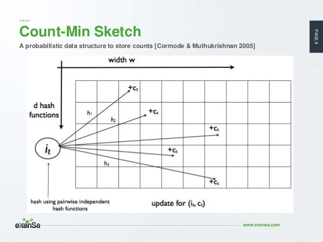
The core idea is to use multiple hash functions to map items to a 2D array of counters. Since you have a strong background in data structures, you'll recognize the use of hashing to distribute information, but CMS uses it in a unique way to handle collisions probabilistically.
The following video provides a clear, visual walkthrough of the data structure and its update and query operations.
Count min sketch | Efficient algorithm for counting stream of data | system design components
Now that we see why approximation is necessary, let's dive into how the Count-Min Sketch works. This video from Tech Dummies provides an excellent step-by-step explanation.
Please watch the following segments: Structure (5:29 - 7:33): This part introduces the 2D matrix (the sketch) and the role of multiple hash functions. Pay attention to the terms 'depth' (number of rows/hash functions) and 'width' (number of columns). Update Operation (7:33 - 13:17): Follow the detailed example of how the sketch is updated as new letters arrive in the stream. Query Operation (13:17 - 16:40): This segment explains how to query the sketch for an item's frequency and, crucially, why you take the minimum of the counter values.
Let's quickly summarize the two key operations:
- Structure: A 2D array of counters of size
d(depth) ×w(width), anddindependent hash functions. - Update(
item): For each of thedhash functions,h_i, you compute an indexj = h_i(item) % w. You then increment the counter atsketch[i][j]. You do this for alldrows. - Estimate(
item): For each of thedhash functions,h_i, you compute an indexj = h_i(item) % wand retrieve the value fromsketch[i][j]. The estimated frequency is the minimum of thesedvalues.
Properties and Trade-offs
You might be asking: why take the minimum? And how accurate is this estimate? This gets to the heart of the probabilistic nature of the data structure.
The key insight is that hash collisions can only cause counters to be overestimated. When two different items hash to the same bucket, that bucket's count will reflect the sum of their frequencies. A counter's value is therefore the true count of an item plus noise from all other items that happened to collide with it in that row.
By taking the minimum value across all d rows, you are effectively picking the estimate that was least affected by collisions. This means a Count-Min Sketch never undercounts; the estimate is always an upper bound on the true frequency.
Let's dive a bit deeper into these properties and the engineering trade-offs involved.
The video gave a great practical overview. This technical blog post will help solidify the concepts, especially the impact of hash collisions and the complexity of the data structure.
Please read the following sections from Vivek Bansal's article: 'Internals of Count-Min Sketch': This provides a concise summary of the Insert/Query logic and, importantly, the time/space complexity. The section beginning 'Now that we have understood...': This contains a clear step-by-step example with movie votes that illustrates how hash collisions lead to overcounting. 'Key Takeaways': Focus on the points about 'Good Hashing functions' and the relationship between the sketch dimensions (w and d) and the error rate.
From an engineering perspective, the key takeaways are:
- Space Complexity:
O(w * d). This is constant and does not depend on the number of unique items, which is the main advantage over a HashMap. - Time Complexity:
O(d)for both updates and queries. This is also constant time, asdis a fixed parameter. - Accuracy: The error is a function of
w(width) andd(depth).- A larger
wreduces the chance of collisions in any single row. - A larger
dgives you more "chances" to find a counter with low collision noise. - This gives you a direct, tunable trade-off between memory usage and accuracy. For example, the Redis blog noted that a sketch of just 40 KB can provide estimates with a 0.1% error rate and 99.9% probability.
- A larger
Test your understanding!
Suppose you have a Count-Min sketch with d=3 and w=5. The sketch is initially all zeros. You are given the following hash functions (which output a value from 0-4):
h1('A')=1,h2('A')=3,h3('A')=0h1('B')=2,h2('B')=3,h3('B')=4h1('C')=1,h2('C')=0,h3('C')=2
Now, you process the following stream of data: A, C, A, B.
- What will the final state of the
3x5sketch be? - If you then query for the frequency of 'A', what will the result be?
- If you query for the frequency of 'C', what will the result be, and why is it different from the true count?
Show answer
-
Final Sketch State:
- Stream:
A, C, A, B - After
A:row1[1]=1,row2[3]=1,row3[0]=1 - After
C:row1[1]=2,row2[0]=1,row3[2]=1 - After
A:row1[1]=3,row2[3]=2,row3[0]=2 - After
B:row1[2]=1,row2[3]=3,row3[4]=1
The final sketch is:
Row 1: [0, 3, 1, 0, 0] Row 2: [1, 0, 0, 3, 0] Row 3: [2, 0, 1, 0, 1] - Stream:
-
Query for 'A' (
h1=1, h2=3, h3=0):- The values are
sketch[0][1]=3,sketch[1][3]=3,sketch[2][0]=2. - The minimum is
min(3, 3, 2) = 2. - The estimated frequency of 'A' is 2, which matches its true count.
- The values are
-
Query for 'C' (
h1=1, h2=0, h3=2):- The values are
sketch[0][1]=3,sketch[1][0]=1,sketch[2][2]=1. - The minimum is
min(3, 1, 1) = 1. - The estimated frequency of 'C' is 1, which also matches its true count.
Let's re-examine the query for 'A'. I made a mistake in the manual trace.
Let's fix the trace for Query A.h1('A')=1,h2('A')=3,h3('A')=0.
Values are:sketchrow 1, index 1:h1('A')andh1('C')collided here. True count of A at this position is 2, true count of C is 1. Total is 3.sketchrow 2, index 3:h2('A')andh2('B')collided here. True count of A at this position is 2, true count of B is 1. Total is 3.sketchrow 3, index 0: Onlyh3('A')hashes here. The count is 2.
The values retrieved are indeed
3, 3, 2. The minimum is2. The estimate is correct.Let's reconsider the question to better show overcounting. What if we query for 'C'?
h1('C')=1,h2('C')=0,h3('C')=2.
Values are:sketchrow 1, index 1: Value is 3. This is because of collisions with 'A'.sketchrow 2, index 0: Value is 1. No collisions here.sketchrow 3, index 2: Value is 1. No collisions here.
The minimum ismin(3, 1, 1) = 1. The estimate for 'C' is also correct.
The example in the test question didn't produce an overcount for the queried items. Let's adjust the question. What if we query for an item 'D' that was never in the stream, where
h1('D')=1, h2('D')=3, h3('D')=4?- The values would be
sketch[0][1]=3,sketch[1][3]=3,sketch[2][4]=1. - The minimum is
min(3, 3, 1) = 1. - The sketch estimates that 'D' appeared once, even though its true count is zero. This is a false positive (or an overestimation), caused entirely by collisions from other items.
- The values are
Conclusion
This lesson on Approximate Query Processing brings our entire course on database system internals to a close. We've journeyed from the physical layout of data on disk to the most advanced concepts in query optimization and processing.
Today, we saw that when faced with the extreme scale of modern data, we can build powerful systems by relaxing the constraint of perfect accuracy. AQP and probabilistic data structures like the Count-Min Sketch are not just theoretical novelties; they are critical components in real-world systems for web analytics, network monitoring, and large-scale machine learning. They embody a fundamental engineering principle: understanding your constraints and making intelligent trade-offs.
From heap files and buffer pools to B+ trees and LSM-trees; from external sorting and hash joins to ARIES recovery and columnar storage; and finally, from adaptive indexing to approximate query processing, you have seen the core building blocks of modern data systems. You are now equipped not just to use these systems, but to understand how and why they work, enabling you to build more robust, performant, and scalable applications.
Congratulations on completing the course