Clustered vs. Unclustered Indexes: Query Performance Impact

Hello! In our last lesson, we saw how B+ Trees enable fast point and range queries and took a first look at how the physical data layout—clustered vs. unclustered—impacts I/O cost. Let's dive deeper into that critical topic.

Introduction

Previously, you learned to traverse a B+ Tree to find specific records and to use the leaf-node sibling pointers for efficient range scans. We ended with a crucial distinction: whether the index leaf nodes store the data itself (clustered) or just pointers to it (unclustered).

Today, we will focus entirely on that distinction. The learning outcome is to compare the impact of clustered versus unclustered B+ tree indexes on query performance. We'll move beyond the basic definitions to analyze performance trade-offs for different types of queries, discuss the concept of "covering indexes," and consider the maintenance overhead for writes. Understanding this is fundamental to designing and tuning high-performance database systems.

1. The Core Difference: A Visual Comparison

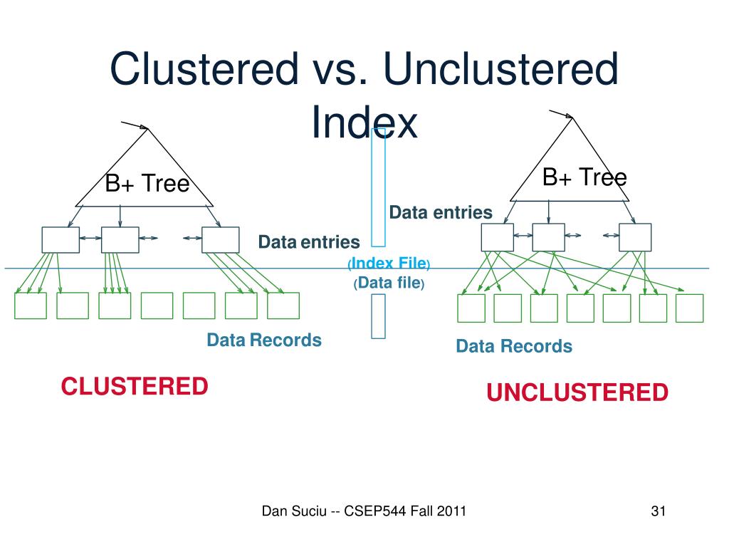
Let's start by solidifying our mental model of these two index types. At its heart, the difference is about physical data locality.

A clustered index determines the physical sort order of data in the table. The leaf nodes of the index and the data are one and the same. Think of it like a dictionary, where the words (the data) are physically sorted alphabetically (the index order). Because a table can only be physically sorted in one way, you can only have one clustered index per table.
An unclustered index is a separate data structure that has its own sorted order, but the actual table data resides elsewhere in an unsorted heap or is sorted by a different (clustered) index. The leaf nodes contain pointers (Record IDs) to the data records. Think of this as the index at the back of a textbook; it's sorted alphabetically, but the page numbers it points to can be all over the book. You can have many unclustered indexes on a table.

Clustered vs. Unclustered Index — This image shows the structural difference. In a clustered index, the data entries in the B+ tree's leaves are the data records themselves, stored in order. In an unclustered index, the data entries are pointers to the data records, which can be stored in any order in a separate data file.

To see this explained with clear animations and a summary of the trade-offs, the following video is an excellent resource.

SQL Indexes (Visually Explained) | Clustered vs Nonclustered | #SQL Course 35

This video provides a clear, visual explanation that contrasts the structure and behavior of clustered and non-clustered indexes. It's a great way to reinforce the core concepts.

Please watch the segment from 20:09 to 28:55. As you watch, focus on the table comparing: The structure (data at leaf level vs. pointers at leaf level). The number of indexes allowed per table. Read vs. Write performance trade-offs. Storage efficiency. Ideal use cases for each type.

2. Analyzing the I/O Performance Impact

As the video highlighted, the structural differences lead directly to performance differences. Let's analyze this from the perspective of disk I/O, which is the dominant cost for large datasets.

The Best Case for Clustered Indexes: Range Scans

Imagine a query that needs to retrieve many rows in a sequence, like fetching all orders for a given month.

With a clustered index on the date column, all the relevant rows are physically next to each other on disk. After the B+ tree traversal finds the first record, the database can simply read the subsequent data pages sequentially. This is highly efficient, costing roughly 1 I/O per page of records.
With an unclustered index, the leaf nodes are sorted, but the data records they point to could be scattered across thousands of different pages on disk. This can lead to a huge number of random I/O operations—one for each record in the worst case. This is inefficient, potentially costing 1 I/O per record.

The following clip from the CMU Database Systems course perfectly illustrates this "random I/O" problem for unclustered indexes and mentions a common optimization databases use to mitigate it.

#08 - Tree Indexes: B+Trees (CMU Intro to Database Systems)

Let's dig deeper into the I/O patterns for range scans. This clip explains why a clustered index enables efficient sequential I/O, while an unclustered index can result in costly random I/O.

Watch the section from 55:56 to 59:00. Pay close attention to: The diagram showing how pointers from an unclustered index can jump all over the heap file pages. The 'thrashing' effect in the buffer pool when using an unclustered index for a large scan. The optimization he describes (sorting record IDs before fetching), which PostgreSQL calls a 'Bitmap Heap Scan'.

The Exception: "Covering" Unclustered Indexes

It might seem like clustered indexes are always better for reads, but that's not true. Consider a query that only needs data available within the index itself. For example: SELECT user_id, registration_date FROM users WHERE registration_date > '2023-01-01'.

If you have an unclustered index on (registration_date, user_id), the database can answer the entire query just by scanning the index leaf pages. It never needs to do the second lookup to the data pages because all the requested columns (user_id, registration_date) are covered by the index.

This is where a "skinny" unclustered index can beat a "fat" clustered index.

The clustered index leaf pages contain all columns of the table, making each page hold fewer rows.
A covering unclustered index contains only a few columns, so its pages are denser, holding many more entries per page.

To satisfy the query, the database has to scan fewer total pages when using the skinny, covering unclustered index. This is a crucial performance tuning concept.

This technical blog post from an industry expert demonstrates this exact scenario.

Performance Myths : Clustered vs. Non-Clustered Indexes

It's a common misconception that a clustered index is always faster for reads. This blog post debunks that myth, showing how a 'skinny' non-clustered index can outperform the 'fat' clustered index for covering queries.

Please read the introduction and the first main example section (up to the discussion of creating a new unique index). Focus on: The COUNT(*) query example, which is a classic covering query. The comparison of logical reads (I/O cost) between the plan using the non-clustered index and the one forced to use the clustered index. The reason for the performance difference: the non-clustered index is 'skinnier' and has fewer total pages to scan.

3. Summary of Performance Trade-offs

Let's summarize the key performance characteristics in a table.

Query Type	Clustered Index Performance	Unclustered Index Performance	Why the Difference?
Point Query (e.g., `WHERE id = 123`)	Excellent. Tree traversal to the leaf page finds the data directly. `~height` I/Os.	Excellent. Tree traversal plus one extra I/O to fetch the data record via its pointer. `~height + 1` I/Os.	The unclustered index requires one extra "hop" to the data page, but this is often a minor difference for a single lookup.
Range Query (e.g., `WHERE date BETWEEN ...`)	Excellent. Reads data pages sequentially from disk. ~1 I/O per page of records.	Potentially Poor. Can lead to random disk I/O. Up to ~1 I/O per record.	Physical data layout. Clustered indexes guarantee data locality for range scans.
Covering Query (e.g., `SELECT key FROM ...`)	Good. Scans all leaf pages, which are wide as they contain all columns.	Often Excellent. Scans a "skinny" index with dense pages, resulting in fewer total I/Os.	A skinny covering index is smaller and requires less I/O to scan than the full clustered index.
Writes (Inserts/Updates/Deletes)	Slower. Inserts may require physically re-ordering data and splitting data pages.	Faster (for the data file). Inserts can be appended to the heap. However, all non-clustered indexes must be updated.	A clustered index enforces physical order, which is expensive to maintain. Write cost increases with the number of indexes on a table.

Test your understanding!

You have a large transactions table with columns (transaction_id PK, user_id, amount, transaction_time, ...) and a clustered index on transaction_id. You are optimizing for two new, frequent queries:

Q1 (Monthly Report): SELECT transaction_id, user_id, amount FROM transactions WHERE transaction_time BETWEEN '2023-01-01' AND '2023-01-31';
Q2 (Quick Total): SELECT SUM(amount) FROM transactions WHERE user_id = 500;

Which type of secondary index (clustered is already taken) would you create for each query to maximize performance, and why?

Show answer

For Q1 (Monthly Report): An unclustered index on transaction_time is the best choice. While this is a range query that will suffer from some random I/O when fetching the full records, it's the only option since a clustered index already exists. Creating the index (transaction_time) will allow the database to quickly find the leaf node pointers for the relevant transactions without scanning the whole table. An optimization like the Bitmap Heap Scan we learned about would then make fetching the data more efficient.
For Q2 (Quick Total): The best choice is a covering unclustered index on (user_id, amount). A query for user_id = 500 will be a point lookup in this index. More importantly, because the amount column is also in the index, the database can calculate SUM(amount) by only looking at the index entries. It never needs to touch the main table data pages. This avoids the +1 I/O hop for every matching record, making it extremely efficient.

Conclusion

You now have a much more nuanced understanding of how clustered and unclustered indexes affect query performance. The choice is not always simple and involves analyzing your specific query patterns and data access needs.

Key Takeaways:

Clustered indexes organize the physical data, making them ideal for range queries where data locality is paramount. You can only have one.
Unclustered indexes are separate pointer structures. While potentially slow for wide range scans that fetch many columns, they are flexible (you can have many) and highly effective for point lookups.
The concept of a covering index is a powerful optimization, where a "skinny" unclustered index can outperform a "fat" clustered index by satisfying a query without touching the main table data, minimizing I/O.
There is always a read/write trade-off. Indexes speed up reads but add overhead to every write operation, as the index structures must be maintained.

Preview of the Next Lesson:

We have spent a lot of time on B+ Trees, the dominant structure for ordered data access. In the next lesson, we will switch gears to another major class of indexing structures: hash indexes. We will start by implementing and analyzing an extendible hashing scheme, a dynamic hashing method designed to grow gracefully as data is inserted, and compare its performance characteristics to the B+ Tree.

Recommended resources