Extendible Hashing: Implementation and Directory Management

Introduction

This lesson focuses on a fundamental dynamic hashing algorithm called extendible hashing. The learning outcome is to implement and analyze an extendible hashing scheme, including directory management.

Unlike static hashing schemes which require costly full-table reorganizations to grow, extendible hashing is designed to expand gracefully as your data scales. We'll explore the clever data structures that make this possible—the directory and buckets—and analyze the algorithms for insertion, splitting, and directory growth. By the end, you'll understand the mechanics of this scheme and the design considerations for a disk-based implementation.

1. From Static to Dynamic Hashing

If you've encountered hash tables in a standard data structures course, you've likely seen static hashing schemes like linear probing or simple chaining. In these schemes, the table has a fixed size. If it fills up, the only solution is to allocate a new, larger table and re-hash every single key. For a database with billions of records, this is prohibitively expensive.

Dynamic hashing schemes, like extendible hashing, solve this problem by allowing the hash table to grow incrementally.

Let's begin by watching a video that clearly explains the core components and logic of extendible hashing.

2. The Core Mechanism: Global vs. Local Depth

As the video explained, the magic of extendible hashing lies in the interplay between the global depth of the directory and the local depth of the buckets.

Let's break down the rules for insertions that cause a bucket to overflow:

1. Find the Target Bucket: Hash the key, take the first g (global depth) bits of the hash value to get an index into the directory, and follow the pointer to the target bucket B.

2. Check for Space: If bucket B has space, insert the key and you're done.

3. Handle Overflow: If bucket B is full, you must split it. Let the local depth of B be l.

   • Case 1: l < g (Simple Split)

     • This is the easy case. Multiple directory entries point to B.
     • Create a new bucket B'.
     • Set the local depth of both B and B' to l + 1.
     • Re-distribute the keys from the original bucket B (plus the new key) between B and B' based on the (l+1)-th bit of their hash values.
     • Update the directory pointers that used to point to B to now point to either B or B' based on that same (l+1)-th bit. The directory itself does not change size.

   • Case 2: l == g (Directory Split)

     • This is the more complex case. Only one directory entry points to B. Splitting the bucket requires us to first expand the directory so we have more pointers to work with.
     • Double the directory size and increment the global depth: g = g + 1. All old pointers are copied over. For example, the old entry 010 now corresponds to new entries 0010 and 1010, which both initially point to the same old bucket.
     • Now that l < g, you can proceed as in Case 1: create a new bucket B', update local depths, redistribute keys, and update the pointers in the newly expanded directory.

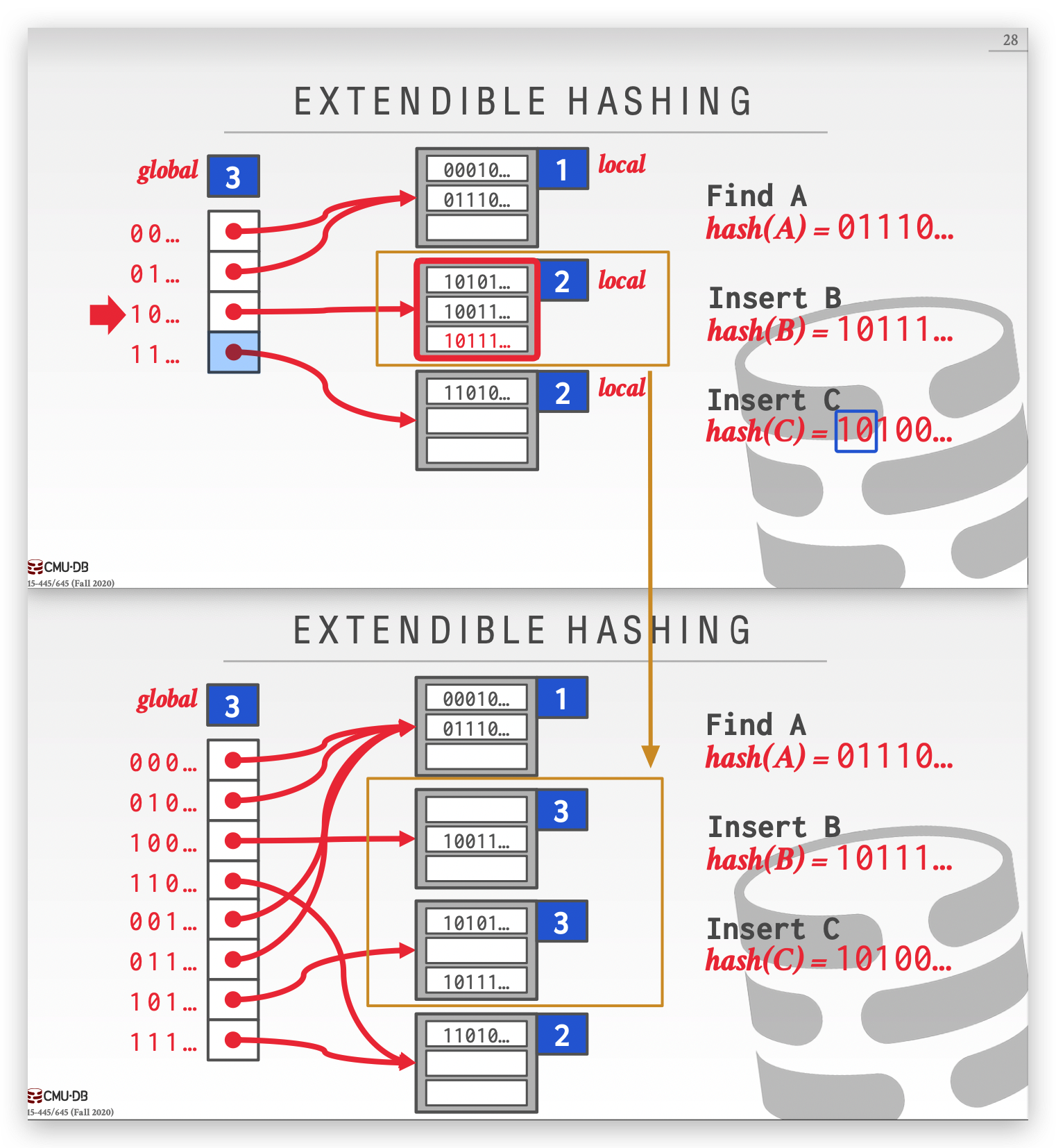
For a more dynamic walkthrough, the following segment from the CMU Database Systems lecture provides excellent animations of these splitting procedures.

3. Implementing a Disk-Based Extendible Hash Index

Your goal is to understand how to implement this scheme. For a disk-based database, this means managing the directory and buckets as pages that are read from and written to disk via the buffer pool.

The CMU Database Systems course includes a project to build exactly this. We won't be implementing it right now, but studying its design specification is invaluable for understanding the practical engineering details.

The specification provides a clear blueprint. The logic described—splitting buckets, growing the directory, and merging on deletion—directly maps to the concepts we've discussed. This mapping from algorithm to a page-based, on-disk implementation is a core skill in database systems engineering.

4. Analysis and Comparison

Now that you understand the mechanics, let's analyze the I/O cost and compare it to B+ Trees.

• Point Lookup: A lookup usually costs 2 I/Os: one to fetch the directory page and one to fetch the bucket page. If the directory is small enough to be cached in memory (a common scenario), the cost drops to just 1 I/O. This is often faster than a B+ Tree traversal, which costs height I/Os (typically 3-4).

• Insertion:

  • No Split: 2 I/Os (read directory, read bucket, then write them back).
  • Simple Split (l < g): Requires more I/Os to write the new bucket page and update the directory.
  • Directory Split (l == g): The most expensive case, as you need to write a whole new set of directory pages. However, since the directory doubles in size each time, these events become exponentially less frequent. The cost is amortized over many insertions.

• Major Weakness: Range Queries
  A hash index does not store keys in any meaningful order. A query like SELECT * FROM users WHERE age BETWEEN 30 AND 40 cannot be answered efficiently. You would have to do a full table scan. This is the fundamental trade-off: hash indexes excel at equality-based point lookups (WHERE id = ?) but are useless for range scans, which are a primary strength of B+ Trees.

Conclusion

In this lesson, you've learned how extendible hashing provides a dynamic index structure that grows gracefully without the need for catastrophic, full-table rehashes.

Key Takeaways:

• Structure: Extendible hashing uses a directory of pointers and buckets for data, managed by a global depth and per-bucket local depths.
• Growth: It grows by splitting full buckets. If a bucket's local depth equals the global depth, the directory itself must double in size. This amortizes the cost of resizing.
• Performance: It offers excellent performance for point lookups, often requiring just one or two I/Os.
• Trade-off: Its major limitation is the complete inability to support efficient range queries, making B+ Trees the more versatile, default choice for a general-purpose index.

Preview of the Next Lesson:

Extendible hashing's main complexity is managing the directory. What if we could design a dynamic hashing scheme that doesn't need a directory at all? In our next lesson, we will explore linear hashing, another clever scheme that achieves incremental growth using a simple "split pointer" and multiple hash functions.