B+ Tree Queries: Operations and I/O Analysis

Introduction

In our last lesson, we focused on the dynamic aspects of the B+ Tree, exploring the insertion and deletion algorithms. We saw how node splits and merges work to maintain the tree's crucial invariants: it's always balanced, and every node is at least half-full. You now have a solid understanding of how a B+ Tree can grow and shrink while remaining an efficient data structure.

Today, we'll put that structure to work. Our learning outcome is to perform point and range queries on a B+ tree and analyze their I/O cost. This is the payoff for all the complex insertion/deletion logic. We'll examine how to find a single record (a point query) and how to retrieve a sequence of records (a range query). Most importantly, we'll analyze the performance of these operations by counting disk I/Os, which is the most critical performance metric for a disk-based database.

1. How B+ Tree Searches Work

Every search in a B+ Tree, whether for a single key or a range, begins the same way: by traversing the tree from the root down to a leaf node.

Point Queries (Equality Search)

A point query seeks a single record with a specific key, like WHERE user_id = 123. The algorithm is straightforward:

1. Start at the root page.
2. At each internal node, examine the sorted keys to determine which pointer to follow to get to the next level of the tree. The keys act as "signposts" guiding you down.
3. Repeat this process until you reach a leaf node.
4. Once at the leaf node, perform a search (e.g., binary search) within that node's keys to find the one you're looking for.
5. If the key is found, you retrieve its associated value. This value is typically a Record ID (RID) that points to the full record's location on a data page.
6. If the key is not found in the leaf node, it does not exist in the table.

Range Queries

A range query seeks all records within a given key range, like WHERE age BETWEEN 21 AND 30. This is where the B+ Tree's design truly shines, particularly the linked list structure of its leaf nodes.

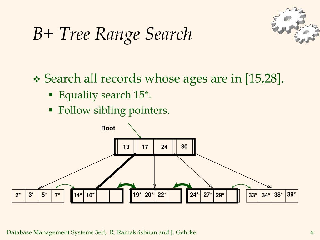
The algorithm for a range query is:

1. Perform a search just like a point query to find the leaf node containing the start of your range.
2. Scan the keys in that leaf node and retrieve the values for all keys that fall within your range.
3. Follow the sibling pointer to the next leaf node.
4. Continue scanning keys and following sibling pointers until you encounter a key that is greater than the end of your range.

This ability to "drop down" into the tree and then perform a fast sequential scan across the ordered leaf nodes is what makes the B+ Tree so powerful for range queries, something a hash index cannot do.

2. Analyzing I/O Cost

In a disk-based database, the primary bottleneck is reading data from disk into memory. CPU operations are orders of magnitude faster. Therefore, we measure the "cost" of a query primarily in terms of the number of disk I/Os required. Each I/O corresponds to fetching one page (which is one node in our B+ Tree) from disk.

I/O Cost of a Point Query

The I/O cost for a point query is the number of pages we must read to find our record.

1. Tree Traversal: The cost is equal to the height of the B+ Tree. A tree of height h requires h I/Os to go from the root to the leaf.
2. Data Fetch: After finding the RID in the leaf node, you need one final I/O to fetch the data page containing the actual record.

So, the total cost is height + 1 I/Os.

A key factor here is the B+ Tree's high fanout (the number of pointers per node). Since the fanout is large (often >100), the height of the tree is very small, even for millions of records. A tree with 300 million records might only have a height of 4!

Furthermore, database systems use a buffer pool to cache frequently accessed pages in memory. The root and upper-level internal nodes of a B+ Tree are almost always in the buffer pool, meaning their I/O cost is often 0.

So, a more realistic I/O cost is: (height - number_of_cached_levels) + 1. In many practical scenarios, this can be just 1 or 2 I/Os.

I/O Cost of a Range Query

The cost of a range query has two components:

1. Tree Traversal Cost: Same as a point query, height I/Os (minus cached pages) to find the first leaf page.
2. Scan Cost: The cost to read the leaf pages that contain the data in the range, plus the cost of reading the actual data pages.

This second component is where things get interesting and depends heavily on how the data is physically organized on disk.

3. Clustered vs. Unclustered Indexes

The I/O cost of fetching the data records for a range query is dramatically affected by whether the index is clustered or unclustered. This is one of the most important concepts in index performance analysis.

As you just read, the distinction is:

• Clustered Index (Alternative 1): The data records are physically sorted on disk in the same order as the index keys. The leaf pages of the B+ Tree essentially are the data file. Since there can only be one physical ordering of a table, you can have only one clustered index per table.

  • Range Query I/O: After traversing to the first leaf, you read pages sequentially. Each data page you read is full of relevant records. The scan cost is approximately 1 I/O per page of matching records. This is highly efficient.

• Unclustered Index (Alternative 2/3): The index is a separate structure where the leaf nodes contain (key, RID) pairs. The RIDs point to data records stored in a heap file, which has a different physical order (e.g., the order they were inserted). You can have many unclustered indexes on a table.

  • Range Query I/O: After traversing to the first leaf, you start scanning the (key, RID) pairs. The RIDs you collect might point to records scattered across many different data pages. In the worst-case scenario, every record you need is on a different page, leading to random disk access. The scan cost is approximately 1 I/O per matching record. This can be very expensive for large ranges.

4. B+ Trees in Action: A PostgreSQL Demo

Theory is great, but seeing how a real database system uses these concepts is even better. The query optimizer's job is to look at a query and decide whether to use an index and, if so, which one. Its decision is based on cost estimates, just like the ones we've been calculating.

This video demonstrates how PostgreSQL's optimizer chooses between a B+ Tree and a hash index for different queries on a table of 27 million email addresses.

The demo highlights the B+ Tree's versatility. It's excellent for equality, excellent for ranges, and can even handle prefix searches, making it the default, all-purpose index structure in most relational databases.

Conclusion

Today we connected the structure of the B+ Tree to its function. By analyzing query algorithms through the lens of I/O cost, the design choices behind the B+ Tree become clear.

Key Takeaways:

• Point queries are highly efficient, costing roughly the height of the tree in I/Os, which is kept low by high fanout and further reduced by buffering.
• Range queries leverage the leaf-node sibling pointers to perform fast sequential scans after an initial traversal.
• The I/O cost of a range query is dominated by the data-fetching step, making the distinction between clustered and unclustered indexes critical.
• Clustered indexes are ideal for range queries, costing ~1 I/O per page of records.
• Unclustered indexes can be expensive for wide ranges, costing up to ~1 I/O per record.
• Real-world database systems use these cost models to decide whether using an index is more efficient than simply scanning the entire table.

Preview of the Next Lesson:

We've now established a solid foundation for how B+ Tree indexes work and how their performance is measured. In the next lesson, we will continue this analysis by comparing the impact of clustered versus unclustered B+ tree indexes on query performance in more depth. We'll explore scenarios where an unclustered index is still a good choice and discuss how the query optimizer weighs these trade-offs.