REINFORCE: Policy Gradients with Sampled Returns

1. The REINFORCE Algorithm

The core idea of REINFORCE is to use Monte Carlo estimation to approximate the expectation in the policy gradient theorem. In simple terms, we run our policy, see how well it did, and then "reinforce" the actions that led to good outcomes.

The following video provides a concise and powerful intuition for how this works.

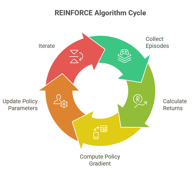
As the video explained, we iteratively update our policy based on the outcomes of sampled trajectories. This entire process can be visualized as a cycle.

Let's formalize this with the algorithm's pseudocode.

The algorithm is as follows:

1. Initialize the policy network ${\pi }_{\theta }$ with random parameters $\theta$.
2. Loop for a number of episodes:
   a. Generate a full trajectory $\tau =(s_0,a_0,r_1,s_1,a_1,\dots ,s_{T-1},a_{T-1},r_T)$ by running the current policy ${\pi }_{\theta }$.
   b. For each timestep $t$ from 0 to $T-1$:
   i. Calculate the return from that step onwards: $G_t={\sum }_{k=t}^{T-1}{\gamma }^{k-t}{r}_{k+1}$. This is the sum of discounted future rewards.
   ii. Update the policy parameters using gradient ascent. The update for the entire episode is a sum of the updates for each timestep:
   $\theta \leftarrow \theta +\alpha {\sum }_{t=0}^{T-1}{G}_t{\nabla }_{\theta }\log {\pi }_{\theta }(a_t|s_t)$

2. Using Sampled Returns for Gradient Estimation

The central part of our learning outcome is understanding how REINFORCE uses sampled returns. The key is the connection between the theoretical action-value function, $Q^{\pi }(s,a)$, and the sampled return, $G_t$.

The policy gradient theorem can also be written using the action-value function $Q^{\pi }(s,a)$:
${\nabla }_{\theta }J(\theta )={\mathbb{E}}_{\pi }[Q^{\pi }(s,a){\nabla }_{\theta }\ln {\pi }_{\theta }(a|s)]$

By definition, $Q^{\pi }(s_t,a_t)$ is the expected return if we start by taking action $a_t$ in state $s_t$ and then follow policy $\pi$ thereafter. The REINFORCE algorithm makes a simple but profound move: it uses the actual return $G_t$ that we observed in a single sampled trajectory as an unbiased Monte Carlo estimate of $Q^{\pi }(s_t,a_t)$.

This is why it's called a Monte Carlo method: we wait until the end of an episode to collect the full sequence of rewards, calculate the returns, and then use these sampled returns to update our policy.

This reading clarifies this crucial substitution.

In essence, the learning process becomes:

1. Try something: Generate a trajectory.
2. See what happened: Calculate the return $G_t$ for each step.
3. Update your strategy: If $G_t$ was high, increase the probability of taking action $a_t$ in state $s_t$. If $G_t$ was low, decrease it. The term ${\nabla }_{\theta }\log {\pi }_{\theta }(a_t|s_t)$ points in the direction to increase the probability of $(a_t|s_t)$, and the return $G_t$ scales how far we step in that direction.

3. A Concrete Example and a Critical Flaw

Now that we understand the mechanics, let's see REINFORCE in action and uncover one of its major limitations. This video first applies the algorithm to a simple 1D problem and then maps the concepts to training a Large Language Model.

The video brilliantly highlights the core weakness of vanilla REINFORCE: high variance. Because a single return $G$ is used to evaluate every action in a trajectory, the gradient estimate can be very noisy. A single bad action can spoil an otherwise good trajectory, unfairly punishing all the good actions. Conversely, a single brilliant action in a mediocre trajectory gets less credit than it deserves.

This "poor credit assignment" makes learning slow and unstable. It's like grading a group project with a single mark—it doesn't reflect individual contributions well.

Conclusion

In this lesson, we translated the Policy Gradient Theorem into the practical REINFORCE algorithm. We saw how it uses Monte Carlo sampling of episode returns to provide an unbiased estimate of the policy gradient, allowing us to directly optimize our policy.

Key Takeaways:

• REINFORCE is a Monte Carlo policy gradient algorithm that updates policy parameters $\theta$ after completing each episode.
• It works by using the sampled return $G_t$ from a trajectory as an estimate of the action-value function $Q^{\pi }(s_t,a_t)$.
• The update rule, $\theta \leftarrow \theta +\alpha G_t{\nabla }_{\theta }\log {\pi }_{\theta }(a_t|s_t)$, effectively "reinforces" actions that led to high returns by making them more probable.
• A major weakness of REINFORCE is high variance due to the credit assignment problem, where every action in a trajectory receives the same reward signal, regardless of its individual contribution.

Preview of the Next Lesson:
The high variance of REINFORCE is a significant problem. How can we fix it? The solution is to judge an action not by the absolute return it achieved, but by how much better or worse that return was compared to what we expected. This leads to the idea of subtracting a baseline. In our next lesson, we will explore how subtracting a baseline from the return significantly reduces variance and stabilizes learning, setting the stage for the powerful actor-critic methods used in modern LLM alignment.