Introduction
Welcome to your next lesson in our Reinforcement Learning module. In our last session, we focused on evaluating a given policy, . We introduced the state-value function, , to measure how good it is to be in a state, and the action-value function, , to measure how good it is to take an action. These are the cornerstones of value-based RL.
Today, we pivot to a more direct approach: policy-based methods. Instead of learning values and then deriving a policy from them, we will directly learn and optimize the policy itself. We'll represent our policy as a parameterized function, , where represents the parameters of a neural network. Our goal is to find the parameters that produce the best possible behavior.
This lesson addresses a fundamental question: How can we use gradient ascent to improve our policy's parameters, , to maximize the expected reward, especially when the reward function is a complex "black box"?
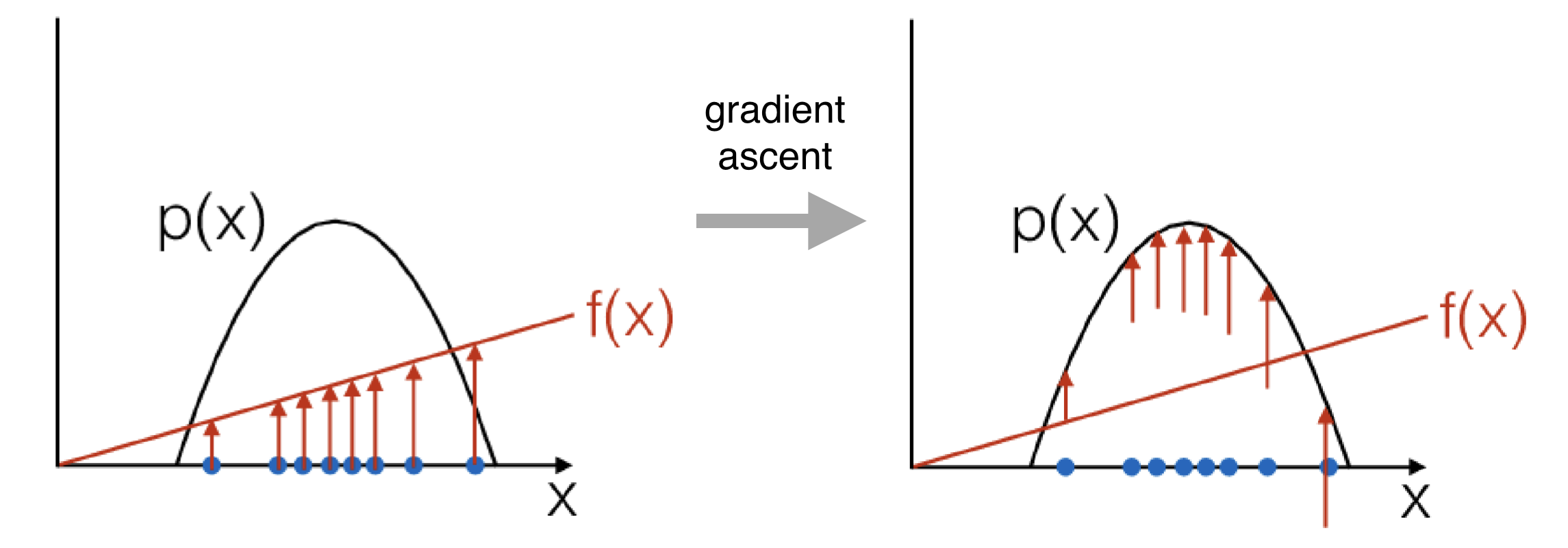
Our learning outcome for this lesson is to state the policy gradient theorem and explain its significance for optimizing parameterized policies. This theorem is the mathematical key that makes direct policy optimization possible.
1. The Challenge: Optimizing with a Black-Box Reward
In supervised learning, you have a clear loss function (like cross-entropy) that you can directly differentiate with respect to your model's weights. In RL, our objective is to maximize the expected total reward, , where is a trajectory generated by our policy .
The problem is that the reward doesn't come from a nice, differentiable function. It comes from interacting with an environment—be it a video game, a physical robot, or even a human providing feedback on an LLM's response. You can't backpropagate a gradient through a game engine or a person's opinion.
This video introduces this core challenge, setting the stage for why we need a new mathematical tool.
To start, let's understand why we need a new tool for this job. Standard gradient descent fails when our reward signal is a 'black box'. This video explains the core problem that policy gradients are designed to solve.
Watch the segments from 00:00 to 01:12 and from 04:49 to 06:00. Focus on why you cannot backpropagate through a black-box reward function, like a human's opinion or a separate reward model used in aligning LLMs.
As the video highlights, the path for gradients is broken. We need a way to estimate the gradient without differentiating the reward function itself.
2. The Policy Gradient Theorem: Derivation and Statement
The Policy Gradient Theorem provides an elegant solution to this problem. It gives us an expression for the policy gradient that we can compute, transforming an intractable problem into a practical one that can be solved with sampling.
The derivation relies on a clever piece of calculus known as the log-derivative trick. This trick allows us to rewrite the gradient in the form of an expectation, which can then be estimated using a Monte Carlo approach (i.e., by averaging over samples from our policy).
The following video provides an excellent, step-by-step derivation.
The solution to this 'black-box' problem is the Policy Gradient Theorem. It provides a mathematical 'trick' to calculate the gradient of our expected reward. This video walks through the derivation, starting with a naive approach that fails and then showing how the 'log-derivative trick' saves the day.
Watch carefully from 06:00 to 10:29. The goal is to follow the derivation from the initial objective function to the final, computable expectation. Pay close attention to why the initial attempt is a 'dead end' and how the log-derivative trick transforms the intractable integral into a sample-based expectation.
To solidify your understanding, let's review the same derivation in a written format from OpenAI's "Spinning Up" series, a highly respected resource in RL education.
Part 3: Intro to Policy Optimization
The video gave an intuitive derivation. Now, let's look at a clear, written derivation from OpenAI's Spinning Up guide. This will solidify the mathematical steps and formally present the simplest form of the policy gradient.
Read the section titled 'Deriving the Simplest Policy Gradient'. Follow the five facts listed and see how they are combined to arrive at the final expectation formula. This is the core statement of the theorem.
The Theorem
As you've now seen in two forms, the Policy Gradient Theorem states that the gradient of the policy performance is:
Let's break this down:
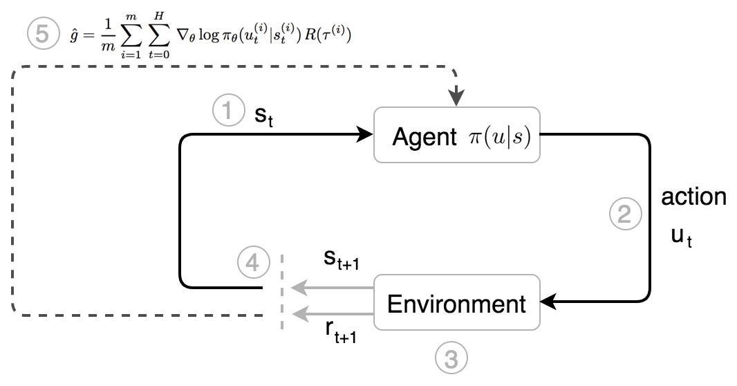
- : This is an expectation over trajectories sampled by running our policy in the environment. This means we can estimate this value by running the policy, collecting a batch of trajectories, and averaging the results.
- : This is the total reward for an entire trajectory . It acts as a weight.
- : This is the gradient of the log-probability of taking action in state . This term is crucial because it's a vector in the parameter space that tells us how to change to make the action more (or less) likely at state .
In short, the theorem tells us that to get the policy gradient, we can sample a trajectory, see what total reward we got, and then nudge our policy parameters to make that entire sequence of actions more likely if the reward was good, and less likely if the reward was bad.
3. The Significance of the Theorem
So, why is this theorem so important? It has three profound implications that unlock modern reinforcement learning.
1. It Makes the Gradient Computable
The most critical contribution is that it transforms an intractable gradient into a sample-based estimate. We don't need to know the inner workings of the environment () or differentiate it. All we need is to be able to:
- Run our policy to generate trajectories.
- Calculate the log-probabilities of the actions we took, , which is a standard output for any probabilistic model like one using a softmax layer.
- Observe the total reward .
This is why policy gradients are so versatile and can be applied to complex environments like video games or robotics simulators.
2. It Provides an Intuitive Update Rule
The formula directly translates to an intuitive learning rule: "reinforce good behavior."
- If is high and positive, the gradient step will increase the log-probabilities of all actions taken in that trajectory.
- If is negative or low, the gradient step will decrease the log-probabilities.
This aligns perfectly with the goal of finding a policy that maximizes reward.
3. It Decouples the Policy from the Environment Dynamics
The gradient calculation, , depends on and the rewards, but not on the gradient of the state distribution, . This is a subtle but vital point. The distribution of states you visit depends on your policy, and if you had to calculate how that distribution changes when your policy changes, the problem would be much harder. The theorem cleverly sidesteps this.
This short reading emphasizes this crucial point.
Policy Gradient Algorithms | Lil'Log
To fully grasp the theorem's importance, let's read a concise explanation that focuses on why the theorem is so powerful.
Read the section 'Policy Gradient Theorem'. The key insight here is that the theorem provides a way to compute the gradient without needing to know the derivative of the state distribution, which is dependent on the unknown environment dynamics. This is the central reason policy gradients are so versatile.
This decoupling is what makes policy gradients a general-purpose tool for optimization in sequential decision-making problems.
Conclusion
In this lesson, we have moved from evaluating policies to directly optimizing them. We confronted the challenge of optimizing for black-box rewards and saw how the Policy Gradient Theorem provides a powerful and elegant solution.
Key Takeaways:
- Policy-based methods directly optimize the parameters of a policy to maximize expected reward.
- The primary challenge is that the reward function is often a non-differentiable "black box," making standard gradient descent impossible.
- The Policy Gradient Theorem provides a computable expression for the gradient of the expected reward:
- Significance: The theorem's main contribution is transforming an intractable analytical gradient into an expectation that can be estimated by sampling trajectories from the policy. This allows us to use gradient ascent to improve policies in any environment where we can run the policy and observe rewards.
Preview of the Next Lesson:
The theorem gives us the gradient, but how do we practically use it in an algorithm? In our next lesson, we will cover the REINFORCE algorithm, the most direct and intuitive implementation of the policy gradient theorem. We will see how it uses sampled episode returns to estimate the policy gradient and update the agent's policy. We will also begin to uncover a major weakness of this simple approach—high variance—which will motivate the more advanced algorithms we will study later, such as PPO and GRPO.