Baseline Subtraction for Variance Reduction in Policy Gradients

Introduction

Welcome back! In our last lesson, we built our first policy gradient algorithm, REINFORCE. We saw that it directly optimizes the policy by increasing the probabilities of actions that lead to high returns, using the update rule:

θ \leftarrow θ + α G_{t} \nabla_{θ} lo g π_{θ} (a_{t} ∣ s_{t})

However, we also identified a critical flaw: high variance. Because the sampled return $G_{t}$ can vary wildly from one episode to the next, the gradient estimates are noisy, making learning unstable and slow. If all rewards in an episode happen to be positive, REINFORCE will reinforce all actions taken, even the suboptimal ones.

This lesson directly addresses that problem. Our learning outcome is to explain how subtracting a baseline reduces variance in policy gradient estimates. This simple but powerful technique is fundamental to making policy gradient methods practical and forms the conceptual bridge to the advanced actor-critic algorithms we'll see later in the course, like PPO.

1. The Problem: Why High Variance Slows Learning

To build a strong intuition for the problem, let's consider an environment where the returns are always positive. This could happen if, for example, all rewards were shifted upwards by a constant.

The following video demonstrates this exact scenario and explains why it's so problematic for the vanilla REINFORCE algorithm.

Policy Gradient Methods | Reinforcement Learning Part 6

This clip from the 'Mutual Information' channel explains the issue with always-positive returns using a simple but effective example.

Watch from 16:40 to 18:07. Focus on the core argument: when the return G_t is always positive, all actions are made more likely. The optimal policy only emerges when the 'really good things' have had a long time to overwhelm the 'pretty good things'.

As the video highlighted, the issue is that the absolute magnitude of the return $G_{t}$ isn't a great learning signal on its own. We don't just want to know if a return was positive; we want to know if it was better or worse than what we expected to get from that state. This is the key idea behind introducing a baseline.

2. The Solution: Subtracting a Baseline

To fix this, we introduce a baseline, $b (s_{t})$ , which is a value that depends only on the current state $s_{t}$ . We then modify the policy gradient update to use the return relative to this baseline.

The new update term becomes:

\nabla_{θ} J (θ) \propto \nabla_{θ} lo g π_{θ} (a_{t} ∣ s_{t}) (G_{t} - b (s_{t}))

Now, the logic is more refined:

If $G_{t} > b (s_{t})$ , the return was better than expected. We reinforce action $a_{t}$ .
If $G_{t} < b (s_{t})$ , the return was worse than expected. We discourage action $a_{t}$ (by pushing the gradient in the negative direction).

This centers the learning signal around zero, providing a much more stable and informative gradient.

3. Is This Mathematically Sound? The Unbiased Property

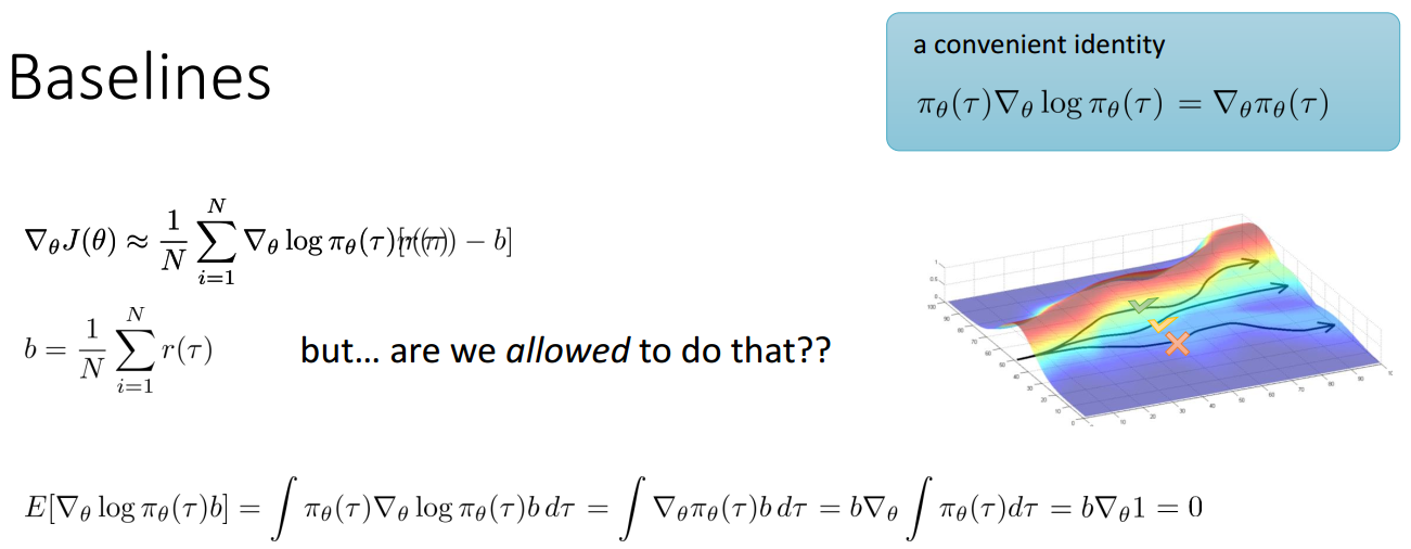
Your first question might be: can we just subtract an arbitrary state-dependent function without messing up the math? The answer, fortunately, is yes. Subtracting a baseline $b (s_{t})$ does not introduce any bias into our gradient estimate. The expected value of the gradient remains the same.

Let's look at the mathematical proof, which relies on the log-derivative trick we saw in the previous lesson.

Baselines for Policy Gradient Variance Reduction

This brief reading from ApX Machine Learning provides a concise proof demonstrating that a state-dependent baseline is an unbiased addition to the policy gradient update.

Read the section under the heading 'Baselines for Variance Reduction', focusing on the mathematical derivation showing that the expected value of the subtracted term is zero. This is a crucial piece of theory.

The key steps in the proof are:

We need to show that the expectation of the term we're subtracting is zero: $E_{π_{θ}} [\nabla_{θ} lo g π (a_{t} ∣ s_{t}) b (s_{t})] = 0$ .
Using the log-derivative trick ( $\nabla lo g f (x) = \frac{\nabla f ( x )}{f ( x )}$ ), we rewrite $\nabla_{θ} lo g π (a_{t} ∣ s_{t})$ as $\frac{\nabla _{θ} π ( a _{t} ∣ s _{t} )}{π ( a _{t} ∣ s _{t} )}$ .
The expectation involves summing over all states and actions, weighted by their probabilities. The $π (a_{t} ∣ s_{t})$ terms cancel out.
We are left with $\sum_{s} d (s) b (s) \nabla_{θ} \sum_{a} π (a ∣ s)$ .
Since the sum of probabilities of all actions from a state is always 1, $\sum_{a} π (a ∣ s) = 1$ .
The gradient of a constant ( $\nabla_{θ} 1$ ) is 0, so the entire expression is 0.

Baselines in Policy Gradient: Variance Reduction and Proof of Unbiasedness — This diagram illustrates the core components of the proof. The term we subtract involves the baseline b(s), which depends only on the state. The proof shows that the expectation of this term is zero, meaning our gradient estimate remains unbiased.

For a more intuitive explanation of why this works, the following video provides a great analogy.

Policy Gradient Theorem Explained - Reinforcement Learning

The math is solid, but what's the intuition? This clip from Elliot Waite explains why subtracting a shared value doesn't change the optimal direction of improvement.

Watch from 50:45 to 52:18. The video explains that subtracting a mean value is like adding a constant negative reward to every possible outcome. Since you can't avoid this 'penalty,' it doesn't change which actions are relatively better or worse, so the direction of the gradient isn't affected on average.

4. Choosing the Right Baseline and Reducing Variance

Now that we know we can use a baseline, what should we use?

The ideal baseline is the state-value function, $V^{π} (s_{t})$ , which is the true expected return from state $s_{t}$ under our current policy $π$ .

Why is this ideal?

It's the most accurate "expectation" to compare our sampled return $G_{t}$ against.
The term $G_{t} - V^{π} (s_{t})$ is an estimate of the Advantage Function, $A^{π} (s_{t}, a_{t}) = Q^{π} (s_{t}, a_{t}) - V^{π} (s_{t})$ . The advantage tells us how much better it was to take action $a_{t}$ compared to the average action from state $s_{t}$ . This is a much more targeted and lower-variance signal than the raw return $G_{t}$ .

Of course, we don't know the true $V^{π} (s_{t})$ . So, in practice, we learn an approximation of it, $V_{w} (s_{t})$ , using a second neural network. This network is often called the Critic, as it "criticizes" the actions chosen by the policy network (the Actor).

The following resources show the dramatic effect of using a baseline.

Policy Gradient Methods in Reinforcement Learning

Let's look at the practical impact. This article from Vizuara's Substack provides a clear comparison of REINFORCE with and without a baseline on the classic CartPole problem.

First, read the code snippet in the 'REINFORCE with Baseline' section, specifically the calc_qvals function, which shows how a simple mean of returns is used as a baseline. Then, observe the two graphs at the end comparing the rewards and Q-value variance for both methods. Notice how the variance is significantly lower and convergence is much faster with the baseline.

The video from Mutual Information that we started with also completes this story by showing the improved performance on the "windy highway" problem.

Policy Gradient Methods | Reinforcement Learning Part 6

Let's return to the 'windy highway' example and see how adding a baseline solves the problem of slow learning.

Watch from 18:07 to 21:27. This part introduces the concept of a baseline (using the state-value function), explains the REINFORCE with Baseline algorithm, and shows a side-by-side comparison of the learning curves. The improvement is striking.

As you can see from both the article and the video, introducing a baseline dramatically reduces the variance of the gradient updates and leads to faster, more stable convergence.

Conclusion

In this lesson, we tackled the high variance problem of the vanilla REINFORCE algorithm. By introducing a state-dependent baseline, we transformed the learning signal from an absolute return to a relative measure of performance, significantly improving learning stability.

Key Takeaways:

Vanilla REINFORCE suffers from high variance because the sampled return $G_{t}$ can be a noisy estimate of an action's quality.
Subtracting a baseline $b (s_{t})$ from the return, $G_{t} - b (s_{t})$ , centers the learning signal. Actions are now judged based on whether they were better or worse than expected.
This modification is unbiased, as the expected value of the subtracted term is zero. It reduces variance without changing the expected gradient direction.
The ideal baseline is the state-value function $V^{π} (s_{t})$ . The term $G_{t} - V^{π} (s_{t})$ serves as an estimate of the advantage function $A^{π} (s_{t}, a_{t})$ .
Since we don't know $V^{π} (s_{t})$ , we learn an approximation of it, which lays the groundwork for Actor-Critic methods.

Preview of the Next Lesson:
We've established that we need to estimate a value function to serve as a baseline. This naturally leads us to a new class of algorithms. In our next lesson, we will formalize this idea by exploring Actor-Critic methods, where one network (the Actor) learns the policy and a second network (the Critic) learns the value function. This architecture is a cornerstone of modern reinforcement learning and a direct precursor to the PPO algorithm used to align models like GPT-4 and DeepSeek-R1.