Unified Embedding Spaces for Multimodal Data

The Core Idea: Creating a Shared Language

In the previous lesson, we learned how a vision encoder produces visual tokens and a text encoder produces text tokens. Initially, these two sets of embeddings exist in completely separate, unaligned vector spaces. An image embedding of a cat is no closer to the text embedding of "cat" than it is to "car" or "planet."

To perform any meaningful cross-modal reasoning, we need to map these representations into a shared embedding space. In this space, the distance and direction between vectors carry semantic meaning, regardless of the original modality.

The pioneering work that established the modern foundation for this was OpenAI's CLIP (Contrastive Language-Image Pre-training).

Contrastive Learning: The Alignment Engine

As the video explained, the key mechanism behind CLIP is contrastive learning. The intuition is simple:

1. Take a large batch of (image, text) pairs.
2. For each image, its correct caption is a positive pair. All other captions in the batch are negative pairs.
3. The model's goal is to maximize the similarity (e.g., cosine similarity or dot product) of embeddings for positive pairs while minimizing the similarity for all negative pairs.

This process effectively "pulls" the embeddings of corresponding images and text descriptions together in the latent space, while "pushing" unrelated pairs apart. The loss function used to achieve this is typically InfoNCE (Noise Contrastive Estimation).

By training on hundreds of millions of pairs, the model learns a robust, generalized embedding space where visual and textual concepts are deeply intertwined.

Extending to Audio and Beyond: A Universal Pattern

The contrastive learning principle is not limited to just text and images. It provides a general recipe for aligning any two modalities for which you can find paired data.

Aligning Audio

How can we bring audio into this shared space? By following the exact same pattern.

As you saw, the process is strikingly similar:

1. Encode Audio: An audio waveform is converted into a spectrogram, and an Audio Spectrogram Transformer (AST) acts as the encoder.
2. Encode Text: A standard text encoder processes the corresponding text caption.
3. Align with Contrastive Loss: A model like CLAP is trained on a massive dataset of (audio, text) pairs to pull their embeddings together in the shared space.

Now, the embedding for the sound of a dog barking is located near the embedding for the image of a dog and the text "a dog barking."

Emergent Alignment with a "Binding" Modality

What if we don't have naturally paired data? For instance, we rarely find datasets of IMU (accelerometer) data paired with text descriptions.

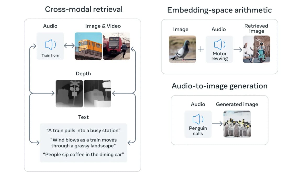
Models like Meta's ImageBind solve this by introducing the concept of a binding modality. Since images are often naturally paired with many other data types (images with text captions, videos with audio, images with depth maps), we can use the image embedding as a common anchor.

By training separate contrastive losses for (Image, Text), (Image, Audio), and (Image, Depth), the model learns to map all these modalities into the same image-centric space. A powerful side effect occurs: emergent alignment. The model learns relationships between modalities that were never explicitly paired in training. For example, it can learn to associate the text "waves crashing" with the audio of waves, because both are independently aligned with images of the ocean.

From Modular Bridges to Native Architectures

This concept of a unified embedding space fundamentally changes how we can build multimodal systems. To understand this shift, let's read a short but critical analysis comparing the old and new paradigms.

As the article explains, we can categorize architectures into two main types:

1. Modular / Late Fusion: This was the previous dominant approach. You have separate, pre-trained encoders for each modality (e.g., a ViT for vision, a text-only LLM for language). A small "projector" or "adapter" module is trained to translate the visual embeddings into the LLM's space. The key issue is that this is a lossy translation; the LLM never sees the "raw" image data, only a compressed, text-aligned summary.

2. Native / Early Fusion: This is the architecture of models like GPT-4o and Gemini. Here, text, image, and audio tokens are all projected into a single, unified embedding space at the input layer. A single, shared Transformer backbone then processes this interleaved sequence of multimodal tokens. This allows for much deeper and more fine-grained interaction between modalities, as attention can flow freely between text, image patches, and audio segments.

The unified embedding space we've been discussing is the essential prerequisite for this more powerful "native" architecture.

Conclusion

In this lesson, we have moved from creating individual visual tokens to understanding how they can be aligned with text, audio, and other modalities in a single, powerful representation.

Key Takeaways:

• A unified embedding space acts as a common semantic "coordinate system" where concepts are represented consistently, regardless of their original modality (text, image, or audio).
• Contrastive learning, powered by loss functions like InfoNCE, is the primary mechanism for creating this space. It trains encoders to pull embeddings of positive pairs (e.g., an image and its correct caption) together while pushing negative pairs apart.
• This pattern is generalizable. CLIP aligns images and text, while CLAP aligns audio and text. Models like ImageBind use a binding modality (images) to create "emergent alignment" between modalities without direct pairing.
• This shared space is the foundation for native multimodal models (like GPT-4o), which fuse modalities at the input layer and process them with a single Transformer, enabling richer cross-modal reasoning than older, modular architectures.

Preview of the Next Lesson:
We have now defined native multimodality and contrasted it with the older, modular approach. In our next lesson, we will perform a deeper comparative analysis, looking at practical examples and performance benchmarks to understand the real-world differences between GPT-4o's native multimodal approach and pipeline-based systems that chain separate models.