Layer-wise Candidate Neighbor Search

The Engine Room: SEARCH-LAYER Algorithm

At its heart, SEARCH-LAYER is a best-first search algorithm. It operates on a single layer of the graph and aims to find the ef nodes closest to a given query vector q. It does this by maintaining a dynamic list of the best candidates found so far and exploring the graph greedily, always prioritizing nodes that are closer to the query.

The original HNSW paper provides the definitive pseudocode for this process. Let's examine it closely.

Let's break down the mechanics of this algorithm.

It manages three key collections of nodes:

1. v (visited elements): A set containing the IDs of nodes whose neighbors have already been considered. This acts like a "closed list" in classic graph search algorithms, preventing the search from getting stuck in loops and re-processing nodes. For an efficient C implementation, a boolean array or a hash set is ideal.
2. C (candidates): A min-priority queue containing nodes that are candidates for exploration. The priority is their distance to the query vector q—the closer a node, the higher its priority.
3. W (found nearest neighbors): A max-priority queue that stores the ef closest nodes found so far. The priority is also the distance to q, but because it's a max-priority queue, the "top" element is always the one furthest from the query. This might seem counterintuitive, but it makes it easy to decide whether a new node is good enough to be added and which old node to discard.

The core of the algorithm is a while loop that runs as long as there are candidates to explore in C.

• Step 1: Extract Best Candidate. In each iteration, it extracts the element c from C that is currently closest to the query q.
• Step 2: Check Stopping Condition. It then compares the distance of c to q with the distance of the furthest element f in the results list W. If distance(c, q) > distance(f, q), the search can stop. This is a critical optimization. It means that the best remaining candidate is already worse than the worst result we've kept. Since we are moving greedily towards the query, we are unlikely to find a better node by exploring from c.
• Step 3: Explore Neighbors. If the search continues, it iterates through all neighbors e of c on the current layer lc.
• Step 4: Update Candidates and Results. For each unvisited neighbor e, it checks if distance(e, q) is smaller than the distance of the furthest element in W (or if W isn't full yet). If it is, e is a valuable find. It's added to the candidates C for future exploration and also inserted into the results W. If adding e makes W exceed its capacity (ef), the furthest element is removed.

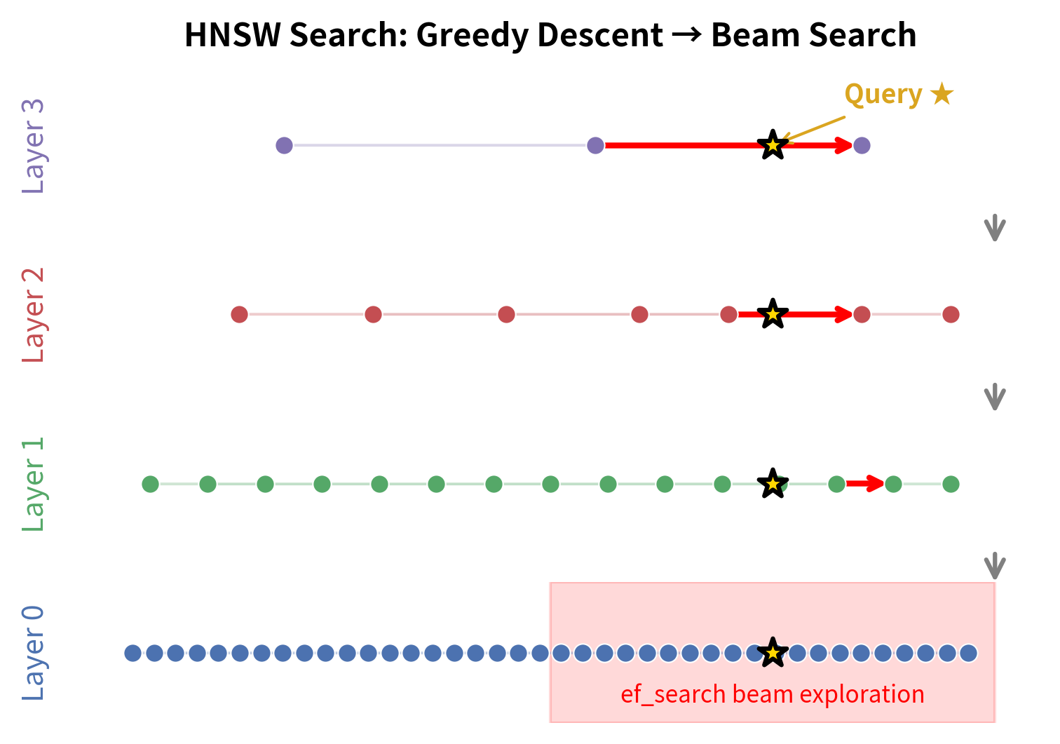
The following diagram, which we've seen before, illustrates the final stage of a search. The "beam exploration" in Layer 0 is precisely the process executed by SEARCH-LAYER.

This video provides a great animated walkthrough of a search, which helps visualize the step-by-step exploration of neighbors within a layer.

The efConstruction Parameter: A Critical Tuning Knob

In the previous lesson, we saw that the INSERT algorithm calls SEARCH-LAYER with two different values for the ef parameter:

1. In Phase 1 (layers L down to l+1): ef is set to 1. This performs a simple greedy search to quickly find the single best entry point for the layer below.
2. In Phase 2 (layers l down to 0): ef is set to efConstruction, a much larger value (e.g., 100 or more).

Why the difference? efConstruction controls the trade-off between graph construction time and search quality.

• A larger efConstruction forces SEARCH-LAYER to maintain a larger list of candidates (W). This means the search is wider and explores more of the local neighborhood. It's more likely to discover diverse, high-quality neighbors that might be slightly further away but are crucial for the graph's "small-world" navigation properties. The result is a better, more robust graph that yields higher search recall. The downside is that graph construction takes longer.
• A smaller efConstruction makes the build process faster but may lead to a lower-quality graph, potentially harming search performance later on.

This parameter is one of the most important tuning knobs in HNSW, allowing you to optimize for your specific use case—for example, a system with frequent updates might favor a faster build, while a static dataset would benefit from a high-quality graph built with a large efConstruction.

C Implementation Sketch

Translating the SEARCH-LAYER pseudocode into C requires implementing the three data structures: the visited set v, the candidate min-priority queue C, and the results max-priority queue W. Given your background, you'll recognize that binary heaps are a natural fit for the priority queues. For the visited set, a simple boolean array is highly efficient if your node IDs are dense, which they will be in our project.

Here is a C skeleton that maps the algorithm's concepts to code. Your task will be to fill in the logic based on the pseudocode.

// Assume we have heap data structures defined:
// MinHeap* min_heap_new();
// void min_heap_push(MinHeap* heap, int node_id, float distance);
// HeapNode min_heap_pop(MinHeap* heap);
//
// MaxHeap* max_heap_new();
// void max_heap_push(MaxHeap* heap, int node_id, float distance);
// HeapNode max_heap_pop(MaxHeap* heap);
// float max_heap_peek_priority(const MaxHeap* heap);

/**
 * @brief Finds the 'ef' nearest neighbors to a query vector on a specific layer.
 *
 * @param hnsw A pointer to the HNSW index.
 * @param query The query vector.
 * @param entry_point_id The ID of the node to start the search from.
 * @param ef The size of the dynamic list of candidates to maintain (efConstruction for insertion).
 * @param layer_idx The layer to perform the search on.
 * @return A MaxHeap containing the 'ef' nearest neighbors found.
 */
MaxHeap* hnsw_search_layer(HNSW* hnsw, const float* query, int entry_point_id, int ef, int layer_idx) {
    // 1. Initialize data structures
    bool* visited = calloc(hnsw->max_elements, sizeof(bool)); // `v`
    MinHeap* candidates = min_heap_new();                     // `C`
    MaxHeap* results = max_heap_new();                         // `W`

    // 2. Add entry point to initial collections
    float dist = hnsw_distance(query, hnsw_get_vector(hnsw, entry_point_id));
    min_heap_push(candidates, entry_point_id, dist);
    max_heap_push(results, entry_point_id, dist);
    visited[entry_point_id] = true;

    // 3. The main search loop
    while (candidates->size > 0) {
        // 4. Extract best candidate 'c' from C
        HeapNode c = min_heap_pop(candidates);

        // 5. Check stopping condition
        float furthest_dist_in_results = max_heap_peek_priority(results);
        if (c.distance > furthest_dist_in_results && results->size >= ef) {
            break; // Optimization: no better candidates left
        }

        // 6. Explore neighbors 'e' of 'c'
        Node* c_node = hnsw_get_node(hnsw, c.id);
        // ... iterate through neighbors of c_node on layer_idx ...
        for (int i = 0; i < c_node->num_connections[layer_idx]; i++) {
            int neighbor_id = c_node->neighbors[layer_idx][i];

            if (!visited[neighbor_id]) {
                visited[neighbor_id] = true;
                
                // 7. Calculate distance and update C and W
                float neighbor_dist = hnsw_distance(query, hnsw_get_vector(hnsw, neighbor_id));

                if (neighbor_dist < furthest_dist_in_results || results->size < ef) {
                    min_heap_push(candidates, neighbor_id, neighbor_dist);
                    max_heap_push(results, neighbor_id, neighbor_dist);
                    
                    if (results->size > ef) {
                        max_heap_pop(results); // Keep results list at size 'ef'
                    }
                }
            }
        }
    }

    free(visited);
    min_heap_free(candidates); // The candidates heap is temporary for the search
    
    // 8. Return the final list of results
    return results; // This is 'W', the set of candidate neighbors
}

Conclusion

You have now completed a deep dive into SEARCH-LAYER, the algorithmic core of the HNSW insertion process. This best-first search, powered by priority queues and a clever stopping condition, is what allows HNSW to efficiently explore the graph and identify promising candidates for connections. You've also seen how the efConstruction parameter provides a powerful lever to control the fundamental trade-off between build time and the quality of the resulting graph structure.

Key Takeaways:

• SEARCH-LAYER is a best-first graph search that uses a min-priority queue for candidates (C) and a max-priority queue for results (W).
• The search is made efficient by a stopping condition: if the best candidate in C is further than the worst result in W, the search can terminate early.
• During insertion, SEARCH-LAYER is called with efConstruction, a large value that ensures a wide search for high-quality, diverse neighbor candidates.
• The set of neighbors W returned by this function is the raw material for the next step in the process.

In our next lesson, we will address that next step: SELECT-NEIGHBORS. Given the large pool of candidates (W) that SEARCH-LAYER has found, how do we intelligently select the best M nodes to form actual connections with? This selection is not based on proximity alone and is key to maintaining the graph's excellent navigational properties.