Neighborhood Selection Heuristic

The Problem with Naive Selection

The simplest way to choose neighbors for our new node q from the candidate pool W would be to pick the M candidates with the smallest distance to q. The HNSW paper calls this SELECT-NEIGHBORS-SIMPLE.

While simple and fast, this approach has a critical flaw. If the new node q lands within a dense cluster of points, its M nearest neighbors will almost certainly all come from that same cluster. This creates a graph with very strong local connections but fails to build the "long-range" links that connect different clusters. A search query can then easily get "trapped" in one region of the graph, unable to find a path to the globally nearest neighbors that might reside in a different cluster.

This image perfectly illustrates the problem and the solution.

In the diagram on the right, the "Inserted element" is much closer to all the blue dots in "Cluster 1" than it is to any dot in "Cluster 2". A naive SELECT-NEIGHBORS-SIMPLE would form connections exclusively within Cluster 1, effectively isolating the new node from the rest of the graph. The heuristic, however, forces the creation of an "extra link" to e_2, creating a vital bridge between the clusters.

This visual comparison makes the difference even clearer:

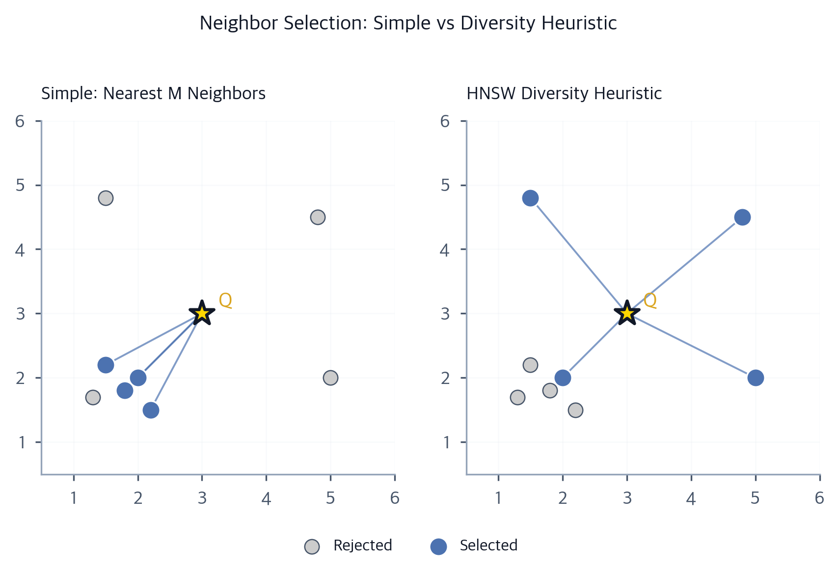
The goal is not just to connect to the closest nodes, but to connect to the most useful nodes for future searches. Usefulness, in this context, means diversity.

The HNSW Neighborhood Selection Heuristic

To build these crucial long-range links, HNSW employs a clever heuristic. The core idea is to favor candidates that offer new directional information. It prunes candidates that are "shielded" by an existing, closer neighbor.

Let's break down the logic as presented in the original paper.

The logic of Algorithm 4 can be summarized as follows:

1. Start with an empty result set R and a working set of candidates W.
2. Iterate through the candidates in W, sorted by their distance to the new node q (from nearest to furthest).
3. For each candidate e, check if it's a "diverse" choice. The paper's condition is: if e is closer to q compared to any element from R. This is most commonly interpreted to mean: dist(q, e) must be less than dist(r, e) for all neighbors r that have already been selected into R.
4. If the condition is met, add e to the result set R. If not, it means e is in the "shadow" of an already-selected neighbor, so we discard it.
5. Continue until we have selected M neighbors or exhausted the candidates.

This process ensures that each new connection we add provides a new "direction" in the vector space, rather than simply reinforcing a connection to a region we've already covered.

The following video from MongoDB gives a great high-level analogy for this. The speaker discusses how the heuristic avoids making redundant connections within a cluster and instead forces the creation of long-range links.

From Algorithm to C Implementation

Now, let's translate this heuristic into a C function. The function will take the candidate pool W (which your hnsw_search_layer function from the last lesson returns as a max-heap), the query vector q, and the target number of neighbors M.

The core challenge is efficiently implementing the check: dist(q, e) < dist(r, e).

Here is a C skeleton for hnsw_select_neighbors_heuristic. Your task is to implement this logic.

#include <stdio.h>
#include <stdlib.h>
#include <stdbool.h>

// Assume these types and functions exist:
// - MaxHeap: The type returned by hnsw_search_layer.
// - HNSW: The main index struct.
// - HeapNode: A struct {int id; float distance;}.
// - hnsw_distance(vec1, vec2): Calculates distance.
// - hnsw_get_vector(hnsw, id): Gets vector for a node ID.
// - A sorting function for HeapNode arrays.

/**
 * @brief Selects M neighbors from a candidate set using the diversity heuristic.
 *
 * @param hnsw A pointer to the HNSW index.
 * @param query The vector for the new node being inserted.
 * @param candidates A MaxHeap of candidate neighbors from SEARCH-LAYER.
 * @param M The number of neighbors to select.
 * @return An array of selected neighbor IDs (callee must free). The size is written to selected_count.
 */
int* hnsw_select_neighbors_heuristic(HNSW* hnsw, const float* query, MaxHeap* candidates, int M, int* selected_count) {
    *selected_count = 0;
    // 1. Convert the max-heap of candidates to a sorted array (min-distance first).
    //    This makes it easy to iterate from the nearest candidate outwards.
    //    For simplicity, you can pop all elements into an array and then sort it.
    int num_candidates = candidates->size;
    HeapNode* sorted_candidates = malloc(num_candidates * sizeof(HeapNode));
    // ... code to populate and sort sorted_candidates ...

    int* results = malloc(M * sizeof(int));
    
    // 2. Iterate through sorted candidates.
    for (int i = 0; i < num_candidates; i++) {
        if (*selected_count >= M) {
            break;
        }

        int candidate_id = sorted_candidates[i].id;
        float dist_query_candidate = sorted_candidates[i].distance;

        bool is_good_candidate = true;

        // 3. For each candidate, check against already selected neighbors.
        for (int j = 0; j < *selected_count; j++) {
            int selected_id = results[j];
            
            // We need the vector for the selected node to calculate the distance.
            const float* selected_vector = hnsw_get_vector(hnsw, selected_id);
            const float* candidate_vector = hnsw_get_vector(hnsw, candidate_id);

            float dist_selected_candidate = hnsw_distance(selected_vector, candidate_vector);

            // 4. This is the core heuristic check!
            if (dist_selected_candidate < dist_query_candidate) {
                is_good_candidate = false;
                break; // This candidate is "shielded" by an existing selection.
            }
        }

        // 5. If it's not shielded, add it to the results.
        if (is_good_candidate) {
            results[*selected_count] = candidate_id;
            (*selected_count)++;
        }
    }

    free(sorted_candidates);
    // Note: The caller is responsible for freeing the `results` array.
    return results;
}

This implementation involves a nested loop, which carries a computational cost. The outer loop runs up to efConstruction times, and the inner loop runs up to M times. This trade-off—a slower, more complex insertion process for a much higher-quality graph—is fundamental to HNSW. The performance cost is justified by the significant gains in search speed and recall later on.

The fast-hnsw library documentation provides a great real-world perspective on this trade-off, referring to the heuristic as PruneStrategy::Heuristic.

Conclusion

In this lesson, you've moved beyond a simple greedy approach to building the HNSW graph. You now understand the critical importance of connection diversity and have the algorithm to achieve it. By favoring neighbors that provide new directional information, this heuristic constructs a graph with robust long-range and short-range links, enabling efficient and accurate navigation.

Key Takeaways:

• Simply selecting the M nearest neighbors (SELECT-NEIGHBORS-SIMPLE) is a flawed strategy that leads to overly clustered graphs and can trap searches in local minima.
• The HNSW diversity heuristic (SELECT-NEIGHBORS-HEURISTIC) solves this by pruning candidate neighbors that are "shielded" by already-selected nodes.
• The core condition for the heuristic is that a new neighbor e is only added if it is closer to the query q than to any neighbor r already in the result set (dist(q, e) < dist(r, e)).
• This process creates a more complex and computationally expensive insertion, but the resulting high-quality graph yields significant improvements in search recall and performance.

In the next lesson, we will take the set of M neighbors you've just selected and physically add the connections to the graph. This involves not only creating the new links but also handling a critical side effect: what to do when adding a connection causes an existing node to exceed its maximum allowed number of neighbors. This will introduce our final core insertion mechanism: connection pruning.