Implementing the HNSW Insertion Algorithm

The Insertion Strategy: From the Top Down

A naive approach to insertion might be to simply find the nearest neighbors on layer l and connect to them. However, HNSW employs a much more sophisticated strategy that is key to its performance. The insertion process always begins at the very top layer of the entire graph, regardless of the new vector's own maximum layer l.

This top-down approach has a significant advantage. The upper layers of the graph are extremely sparse and act as a super-fast "expressway" system. By starting at the top, the algorithm can quickly navigate across vast regions of the vector space to find the rough neighborhood where the new vector belongs. It then progressively refines this search as it moves down through the denser lower layers.

This is analogous to finding a specific address in a large country. You don't start by randomly checking houses. You first navigate to the correct state (top layer), then the correct city (middle layer), and only then do you start searching street-by-street (bottom layer).

The insertion process can be broken down into two distinct phases:

1. Phase 1: Fast Traversal (Above l): From the graph's top layer L down to l+1, the algorithm's only goal is to find the best possible entry point for the layer below. In these layers, we perform a minimal search, looking for just the single nearest neighbor to our new vector.
2. Phase 2: Neighbor Discovery (From l down to 0): Once we reach layer l (the highest layer for our new vector), the mission changes. Now, and for every layer below it, we perform a more exhaustive search to find a set of high-quality candidate neighbors. These are the nodes our new vector will actually connect to.

Let's look at a visualization of this process.

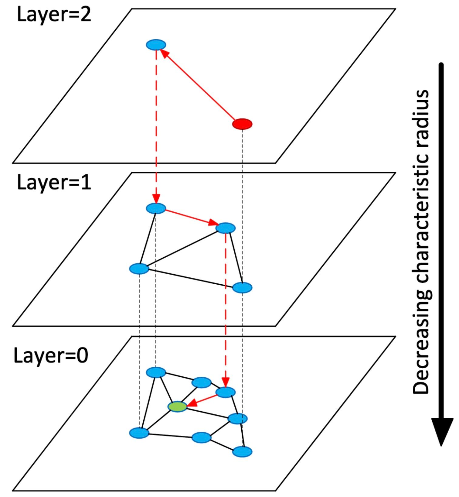
The Formal Algorithm

The original HNSW paper provides the definitive pseudocode for this process. While it looks dense, it maps directly to the two-phase strategy we just discussed.

Let's break down the key lines of Algorithm 1: INSERT(hnsw, q, M, Mmax, efConstruction, mL):

• Line 2-4: Initialize the process. Get the global entry point ep for the graph, find its level L, and calculate the new element's max level l using the function from our last lesson.
• Lines 5-7 (Phase 1): This for loop runs from the top layer L down to l+1. Notice the call to SEARCH-LAYER(q, ep, ef=1, lc). Setting ef=1 is the key here; we are performing the most minimal search possible, just to find the single best node to use as the entry point (ep) for the next layer down.
• Lines 8-10 (Phase 2): This for loop runs from min(L, l) down to 0. Now we are in the layers where the new node q will actually exist. The call to SEARCH-LAYER uses efConstruction, a larger parameter that ensures we find a high-quality, diverse set of candidate neighbors W. Line 10 then passes these candidates to a SELECT-NEIGHBORS function.

The subsequent lines (11-17) deal with creating connections and pruning them if necessary. We will tackle those specific steps in the upcoming lessons. For today, our focus is the main control flow that finds the candidates.

This video provides a great conceptual walkthrough of how the search and insertion processes traverse the hierarchy.

A Detailed Example

Let's trace the insertion of a new blue node, which has been assigned a maximum layer l=2. The graph's highest layer is L=4.

1. Layer 4 (Navigating): The algorithm starts at the global entry point. It performs a SEARCH-LAYER with ef=1 to find the single node on layer 4 closest to our blue node. This node becomes the entry point for layer 3.
2. Layer 3 (Navigating): Starting from the entry point provided by layer 4, the algorithm again runs SEARCH-LAYER with ef=1. It finds the nearest neighbor on layer 3 and uses it as the entry point for layer 2.
3. Layer 2 (Connecting): Now we have reached l=2, the highest layer for our new node. The mission changes. The algorithm runs SEARCH-LAYER with efConstruction (a larger value, e.g., 100) to find a good set of candidate neighbors. From these candidates, a heuristic (SELECT-NEIGHBORS, which we'll build next) chooses the best M neighbors (here, M=2). Bidirectional links are created between the new blue node and these two neighbors. The entire set of candidates found becomes the entry point for the next layer.
4. Layer 1 (Connecting): Using the candidates from layer 2 as entry points, the algorithm again runs SEARCH-LAYER with efConstruction to find candidates on layer 1. It selects the best M=3 neighbors and creates connections.
5. Layer 0 (Connecting): The process repeats one last time on the densest layer. SEARCH-LAYER is called, and the best neighbors (here, M_max0=4) are selected and connected.

The insertion is now complete. For a more concise explanation and pseudocode, this article is also very helpful.

C Implementation Structure

Based on this logic, we can now sketch out the main hnsw_insert function in C. The core of the function will be the two loops we've identified. We will assume the existence of hnsw_search_layer (from Module 6) and stub out the functions for neighbor selection and connection, which we will implement next.

/**
 * @brief Inserts a new vector into the HNSW graph.
 *
 * @param hnsw A pointer to the HNSW index.
 * @param q The vector data for the new element.
 * @param node_id The ID of the new node to be inserted.
 */
void hnsw_insert(HNSW* hnsw, const float* q, int node_id) {
    // A temporary list to hold neighbors found by search_layer.
    // In a real implementation, this would be a min-priority queue or similar.
    CandidateList W = candidate_list_new(); 

    // Get the global entry point and the top layer of the graph.
    int enter_point_id = hnsw->enter_point_id;
    int top_layer = hnsw->max_layer;

    // Step 1: Calculate the random layer for the new element.
    int new_node_layer = hnsw_random_level(hnsw->ml_factor);
    if (new_node_layer > top_layer) {
        // If the new node's layer is higher than the current top layer,
        // it becomes the new entry point. We'll handle this detail later.
    }
    
    // This will be our entry point for the searches on each layer.
    int current_ep_id = enter_point_id;

    // Phase 1: Traverse from the top layer down to the new node's layer + 1.
    // The goal is just to find the best entry point for the lower layers.
    for (int lc = top_layer; lc > new_node_layer; lc--) {
        hnsw_search_layer(hnsw, q, &current_ep_id, 1, 1, lc, &W);
        current_ep_id = candidate_list_get_nearest(W); // Get the single best candidate
        candidate_list_clear(W);
    }

    // Phase 2: From the new node's layer down to 0, find and connect neighbors.
    for (int lc = MIN(top_layer, new_node_layer); lc >= 0; lc--) {
        // Use a more thorough search to find a good set of candidates.
        hnsw_search_layer(hnsw, q, &current_ep_id, 1, hnsw->ef_construction, lc, &W);

        // From the candidate list W, select the M best neighbors.
        NeighborList neighbors = hnsw_select_neighbors(q, W, hnsw->M, lc);

        // Add connections from the new node to its neighbors.
        hnsw_connect_neighbors(hnsw, node_id, neighbors, lc);

        // Prune connections of the neighbors if they exceed M_max.
        // (This will be covered in a future lesson).

        // Use the found candidates as the entry points for the next level down.
        // For simplicity, we just use the best candidate, but using all is better.
        current_ep_id = candidate_list_get_nearest(W); 
        candidate_list_clear(W);
    }

    // Update the graph's metadata (e.g., new top layer, entry point).
    if (new_node_layer > hnsw->max_layer) {
        hnsw->max_layer = new_node_layer;
        hnsw->enter_point_id = node_id;
    }

    candidate_list_free(W);
}

This C code provides the complete skeleton. You have already implemented hnsw_random_level and hnsw_search_layer. The next lessons will focus on filling in the details of hnsw_select_neighbors and hnsw_connect_neighbors.

Conclusion

You have now designed the central control flow for inserting elements into the HNSW graph. This algorithm is the engine of graph construction, and its efficient, top-down design is a masterclass in trading precision for speed at the upper layers to achieve logarithmic performance.

Key Takeaways:

• Top-Down Insertion: The insertion process always starts at the graph's highest layer and descends, ensuring fast navigation through the sparse upper layers.
• Two-Phase Process: The algorithm has two phases: a fast-traversal phase (ef=1) in layers above the new node's level l, and a neighbor-discovery phase (ef=efConstruction) in layers at and below l.
• Reuse of SEARCH-LAYER: The insertion algorithm is built directly on top of the search algorithm, demonstrating excellent code reuse and modularity.
• Entry Point Propagation: The closest node found on one layer becomes the entry point for the search on the layer below, creating a greedy path to the correct neighborhood.

In the next lesson, we will dive into the SELECT-NEIGHBORS heuristic. This is the crucial step where, from a large pool of candidates, we must intelligently choose the best M nodes to connect to, ensuring the graph maintains its "small-world" properties.