Randomized Layer Assignment for Vector Insertion

The Hierarchical Principle: Probabilistic Promotion

The power of HNSW comes from its layered structure, which emulates the logic of a probabilistic skip list. Upper layers are sparse and contain long-range connections for fast, coarse-grained navigation, while the dense bottom layer contains all vectors for fine-grained, accurate search.

To build such a structure, we need a way to decide which nodes belong to which layers. HNSW does this probabilistically: every new node is assigned a maximum layer, l, with an exponentially decaying probability. This means:

• Almost all nodes will be assigned l=0, living only on the bottom layer.
• A small fraction will be "promoted" to l=1, existing on layers 0 and 1.
• An even smaller fraction will reach l=2, and so on.

This random promotion ensures that the number of nodes decreases exponentially with each layer, creating the exact hierarchical pyramid structure we need for logarithmic search complexity. The randomness also makes the graph construction robust and incremental, as it doesn't depend on the order in which vectors are inserted.

The Layer Assignment Formula

This probabilistic assignment is not arbitrary; it's governed by a precise mathematical formula presented in the original HNSW paper. When a new element is inserted, its maximum layer l is chosen as:

$l\leftarrow \lfloor -\ln (\text{unif}(0,1))\cdot m_L\rfloor$

Let's break down this elegant formula, as it's the heart of today's lesson:

1. unif(0,1): We start with a random floating-point number drawn from a uniform distribution between 0 and 1. This is the source of randomness.
2. -ln(...): We take the negative natural logarithm of that random number. In probability theory, this is a standard technique called inverse transform sampling. Applying it to a uniform distribution generates a random variable that follows an exponential distribution. This is the mathematical key to achieving the "exponentially decaying probability" for layer assignments.
3. m_L: This is a normalization factor or "level multiplier". It controls the shape of the exponential decay. A smaller m_L leads to a steeper decay (fewer nodes on higher layers), while a larger m_L leads to a gentler decay (more nodes on higher layers).
4. ⌊...⌋: The floor function simply converts the resulting floating-point value into an integer layer index.

The following interactive resource provides a clear breakdown of this formula and its components. It also includes a concrete example showing the resulting probabilities, which makes the concept much more tangible.

The m_L Normalization Factor

The m_L parameter is not just a magic number; it's directly tied to the connectivity of the graph. The authors of HNSW found that an optimal choice for this parameter is:

$m_L=\frac{1}{\ln (M)}$

Here, M is the parameter that defines the number of neighbors each node will have on a given layer. This creates a beautiful synergy: the probability of a node being promoted to a higher, sparser layer is inversely related to the density of connections on the layers below. A graph with many connections per node (large M) can be navigated effectively even with very sparse upper layers (small m_L).

This entire process is visually summarized in the diagram below and explained well in the following video clip.

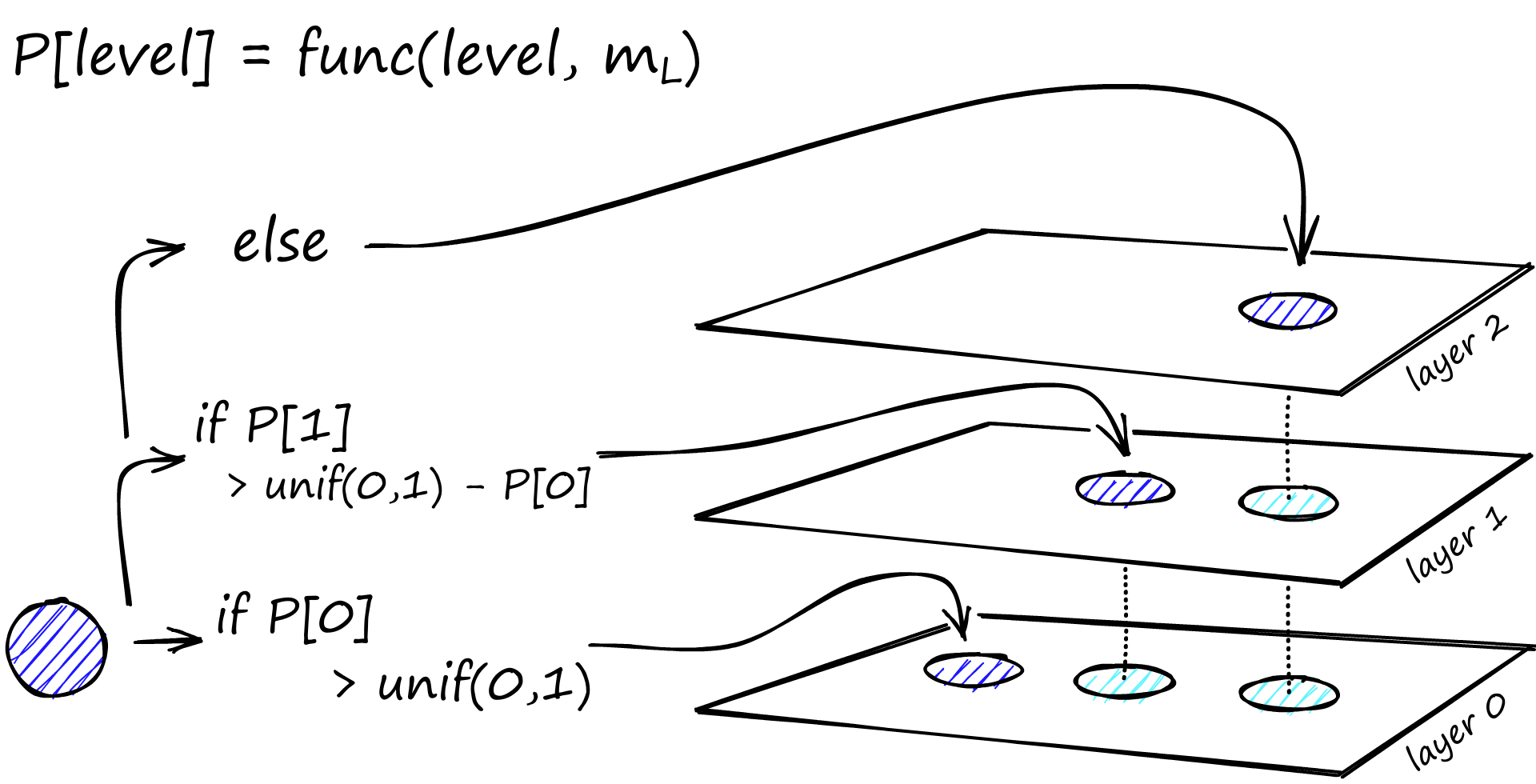
A new node (striped blue) is considered for insertion into the HNSW graph. Its maximum layer is determined probabilistically. It is always added to layer 0, but its presence on higher layers is decided by a series of random trials against an exponentially decaying probability, governed by the m_L factor.

Implementation in C

Now, let's translate this directly into a C function. The implementation is a straightforward application of the formula. We'll need rand() from <stdlib.h> to generate a random number and log() and floor() from <math.h> for the mathematical operations.

Here is a function that implements the logic.

#include <math.h>
#include <stdlib.h>
#include <time.h> // For seeding the random number generator

/**
 * @brief Assigns a random layer to a new element based on an exponential distribution.
 *
 * This function implements the formula l = floor(-ln(uniform(0,1)) * mL)
 * from the HNSW paper. This ensures that the probability of assigning a higher
 * layer decreases exponentially, creating the hierarchical structure.
 *
 * It is crucial to seed the random number generator once at the start of the
 * program (e.g., using srand(time(NULL))) for this function to produce
 * different results on each run.
 *
 * @param ml_factor The normalization factor, calculated as 1.0f / log(M).
 * @return The randomly selected maximum layer for the new element.
 */
int hnsw_random_level(float ml_factor) {
    // Generate a random float in the range (0, 1].
    // We add 1 to rand() and RAND_MAX to avoid the case where rand() is 0,
    // since log(0) is undefined.
    float r = (float)(rand() + 1) / ((float)RAND_MAX + 1);

    // Apply the formula
    float level = -logf(r) * ml_factor;

    return (int)floorf(level);
}

A few notes on this implementation, which are relevant given your background in systems programming:

• Randomness Quality: The standard C rand() function is a pseudo-random number generator (PRNG). While sufficient for this project, production-grade systems often use more robust generators (like those in C++'s <random> library or system-specific sources like /dev/urandom) for better statistical properties.
• Seeding: rand() must be seeded once at the beginning of your program's execution (e.g., in main() with srand(time(NULL))). If you don't seed it, it will produce the same sequence of "random" numbers every time you run the program.
• Floating Point Precision: We use logf and floorf, the single-precision versions of the math functions, as we are working with float types. This can be slightly more performant on some architectures than using the double-precision log and floor.

For a deeper dive, the same video resource shows the presenter analyzing the actual Faiss C++ implementation and replicating its behavior in Python. This is an excellent real-world confirmation of the principles we've discussed.

Conclusion

In this lesson, you've implemented the very first and one of the most elegant components of the HNSW insertion algorithm. By assigning layers probabilistically, the graph builds a robust, efficient hierarchy automatically, without complex rebalancing operations.

Key Takeaways:

• Probabilistic Hierarchy: HNSW uses a random process with an exponentially decaying probability to assign a maximum layer l to each new vector.
• The Core Formula: The assignment is governed by the formula l ← ⌊-ln(unif(0,1)) ∙ m_L⌋, which turns a uniform random number into an exponentially distributed one.
• Tuning with m_L: The m_L parameter, typically set to 1/ln(M), tunes the steepness of the layer hierarchy, linking it to the graph's connection density M.
• C Implementation: The function is a direct and concise translation of the mathematical formula, requiring careful handling of random number generation and floating-point edge cases.

Now that we can determine the maximum layer for a new vector, the next logical step is to find its neighbors and connect it into the graph on each of its assigned layers. In the next lesson, we will implement the main insertion algorithm, which cleverly reuses the SEARCH-LAYER function you built in the previous module to find the best connection points for the new element.