Analyzing Isentropic Devices

The General Toolkit: SFEE and the Isentropic Assumption

Remember the Steady-Flow Energy Equation (SFEE) from Module 5? It's our master equation for analyzing devices with fluid flowing through them. Let's write it down again (on a per-unit-mass basis, using $w$ for work and $q$ for heat):

$q-w=(h_2-h_1)+\frac{V_2^2-V_1^2}{2}+g(z_2-z_1)$

Where:

• $q$ = heat transferred into the system
• $w$ = work done by the system
• $h$ = specific enthalpy (the total energy of the flowing fluid)
• $V$ = velocity
• $z$ = height

For the devices we're studying today (turbines, compressors, nozzles), the change in height is almost always negligible, so we can ignore the $g(z_2-z_1)$ term.

Now, here's the key: we are analyzing ideal devices. As we learned, an ideal process in these devices is an isentropic one. This gives us two powerful simplifications:

1. Adiabatic: The process is perfectly insulated, so there is no heat transfer. This means $q=0$.
2. Reversible: The process is perfectly smooth with no friction, which means the entropy remains constant: $s_2=s_1$.

This second point, $s_2=s_1$, is the magic key that unlocks the whole analysis. It provides the crucial piece of information we need to pinpoint the exact exit state of the fluid.

Let's see how this works for each device.

Analyzing an Ideal (Isentropic) Turbine

A turbine is like a windmill for high-energy fluid. Its job is to extract energy from a flowing fluid (like steam or hot gas) and convert it into rotational work, like turning an electricity generator.

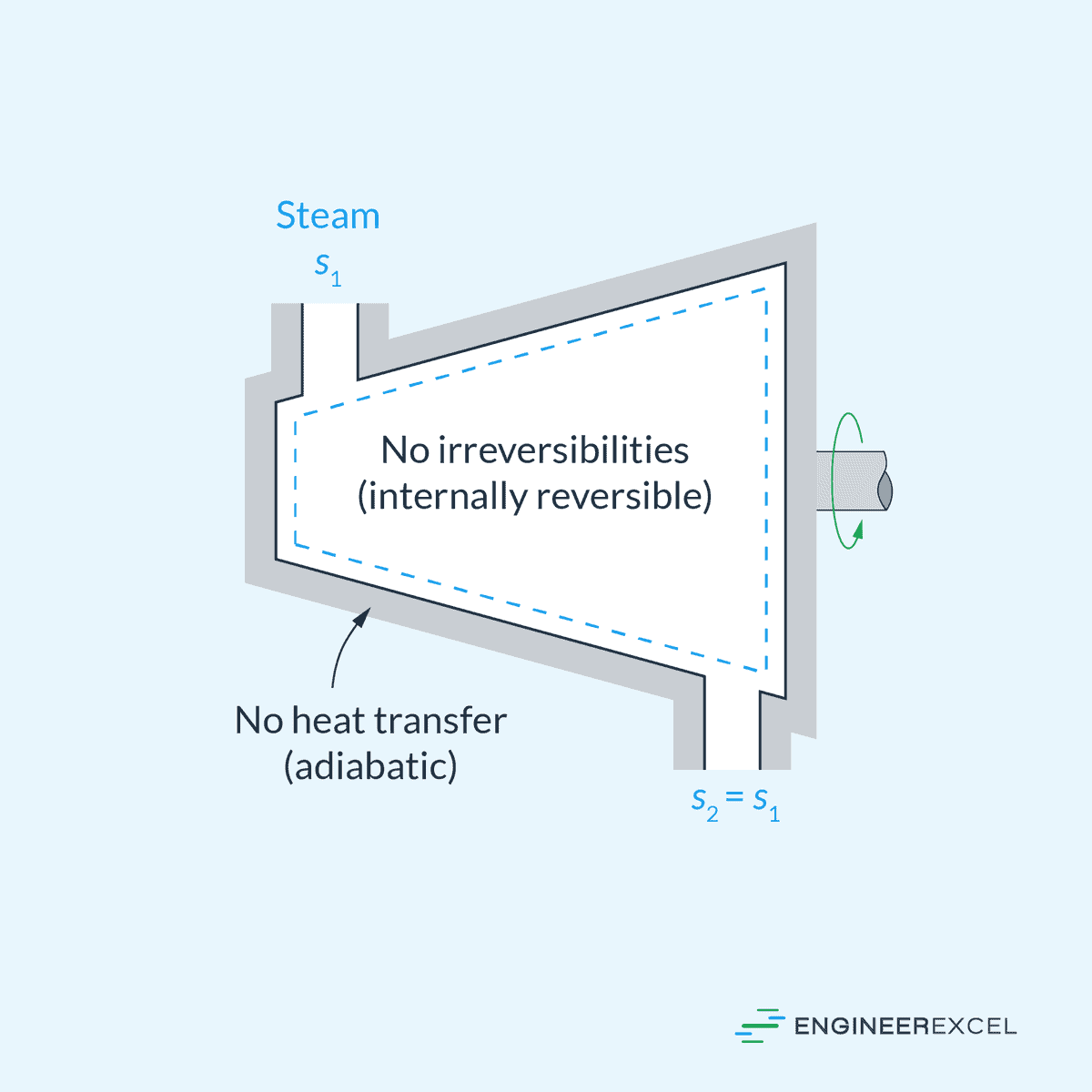
Let's simplify the SFEE for our ideal turbine:

• $q=0$ (it's adiabatic).
• For turbines, the change in kinetic energy is usually tiny compared to the change in enthalpy, so we'll assume $\frac{V_2^2-V_1^2}{2}\approx 0$.

The SFEE boils down to:
$0-w_{turb}=(h_2-h_1)$
$w_{turb,out}=h_1-h_2$

To show that we're talking about the ideal, isentropic case, we'll label the exit state with an 's'. So, the ideal work output is:

$w_{ideal,out}=h_1-h_{2s}$

The big question is: How do we find $h_{2s}$?
We typically know the inlet conditions (State 1: $P_1$, $T_1$) and the pressure the turbine exhausts to (State 2: $P_2$). That's not enough to know the enthalpy $h_2$. But since the process is isentropic, we have our magic key:

$s_{2s}=s_1$

So, the ideal exit state (State 2s) is fixed by two properties: the known exit pressure $P_2$ and the entropy $s_1$ from the inlet.

Example 1: An Ideal Steam Turbine (Using Property Tables)

Let's analyze a steam turbine. Steam is a "real substance," so we have to use steam tables. This process is fantastically illustrated on an enthalpy-entropy (h-s) diagram, also called a Mollier chart.

To learn about this chart and see how it visually represents our turbine process, please read the following material.

Now, let's solve a problem.

Problem: Superheated steam enters an ideal turbine at 5 MPa and 400°C. It expands to a pressure of 40 kPa. What is the work output of the turbine per kg of steam?

Solution:

Step 1: Find properties at the inlet (State 1).
We are given $P_1=5\text{ MPa}$ and $T_1=400^{\circ }\text{C}$. We go to the superheated steam tables.
Looking up at P = 5.0 MPa, we find the row for T = 400°C.

• Enthalpy: $h_1=3196.7\text{ kJ/kg}$
• Entropy: $s_1=6.6483\text{ kJ/kg}\cdot \text{K}$

Step 2: Use the isentropic condition to define the ideal exit state (State 2s).
We know the exit pressure is $P_2=40\text{ kPa}$. The magic key for an ideal turbine is that entropy is constant:
$s_{2s}=s_1=6.6483\text{ kJ/kg}\cdot \text{K}$

So, State 2s is defined by: $P_{2s}=40\text{ kPa}$ and $s_{2s}=6.6483\text{ kJ/kg}\cdot \text{K}$.

Step 3: Find the enthalpy at the ideal exit state (h_2s).
We go to the saturated steam tables at $P=40\text{ kPa}$. We need to figure out if the steam at the exit is still superheated, a saturated mixture, or a compressed liquid.
At 40 kPa, we find the entropies for saturated liquid ($s_f$) and saturated vapor ($s_g$):

• $s_f=1.0261\text{ kJ/kg}\cdot \text{K}$
• $s_g=7.6691\text{ kJ/kg}\cdot \text{K}$

Our entropy, $s_{2s}=6.6483$, is between $s_f$ and $s_g$. This tells us the steam at the exit is a saturated liquid-vapor mixture. We need to find its quality, $x$.

Recall the formula: $s=s_f+x\cdot s_{fg}$, where $s_{fg}=s_g-s_f$.
$s_{fg}$ at 40 kPa is $7.6691-1.0261=6.6430\text{ kJ/kg}\cdot \text{K}$.

$6.6483=1.0261+x_{2s}\cdot (6.6430)$
Solving for $x_{2s}$:
$x_{2s}=\frac{6.6483-1.0261}{6.6430}=0.846$
This means the steam at the ideal exit is 84.6% vapor.

Now we can find the enthalpy $h_{2s}$ using the same quality:
$h_{2s}=h_f+x_{2s}\cdot h_{fg}$
From the table at 40 kPa: $h_f=317.65\text{ kJ/kg}$ and $h_{fg}=2318.4\text{ kJ/kg}$.
$h_{2s}=317.65+0.846\cdot (2318.4)=317.65+1961.3=2278.95\text{ kJ/kg}$

Step 4: Calculate the ideal work output.
$w_{ideal,out}=h_1-h_{2s}=3196.7-2278.95=917.75\text{ kJ/kg}$

This is the maximum possible energy we can extract from each kilogram of steam under these conditions. A real turbine would have friction and produce less work.

To see this exact type of calculation performed using both the tables and a Mollier chart, you can review the following example.

Analyzing an Ideal (Isentropic) Compressor

A compressor does the opposite of a turbine: it takes in work to increase the pressure of a fluid. Think of an air compressor filling a tank or the compressor in your refrigerator.

The simplified SFEE for an ideal compressor is:
$-w_{comp,in}=(h_2-h_1)$
$w_{comp,in}=h_2-h_1$

For the ideal (isentropic) case, this becomes:
$w_{ideal,in}=h_{2s}-h_1$

The logic is identical to the turbine, just in reverse. We know the inlet state ($P_1,T_1$) and the desired outlet pressure ($P_2$). We use our magic key, $s_{2s}=s_1$, to find the ideal exit enthalpy $h_{2s}$ and thus the minimum work required.

Example 2: An Ideal Air Compressor (Using Ideal Gas Relations)

Problem: Air enters an ideal compressor at 100 kPa and 25°C. It is compressed to 800 kPa. What is the minimum work input required? (For air, use $c_p=1.005\text{ kJ/kg}\cdot \text{K}$ and $k=1.4$).

Solution:

Step 1: Convert temperature to Kelvin.
A crucial step whenever using ideal gas laws!
$T_1=25+273.15=298.15\text{ K}$

Step 2: Use the isentropic relation to find the ideal exit temperature (T_2s).
For an ideal gas undergoing an isentropic process, you'll recall this relation from Module 4:
$\frac{T_{2s}}{T_1}={\left(\frac{P_2}{P_1}\right)}^{(k-1)/k}$
Let's calculate the exponent: $(k-1)/k=(1.4-1)/1.4=0.4/1.4\approx 0.2857$.
$T_{2s}=T_1{\left(\frac{P_2}{P_1}\right)}^{0.2857}=298.15\text{ K}{\left(\frac{800\text{ kPa}}{100\text{ kPa}}\right)}^{0.2857}$
$T_{2s}=298.15\cdot (8{)}^{0.2857}=298.15\cdot (1.811)=540.0\text{ K}$
The air gets very hot during this ideal compression, reaching 540 K (or 267°C)!

Step 3: Calculate the ideal work input.
For an ideal gas, the change in enthalpy is simply $\Delta h=c_p\Delta T$.
$w_{ideal,in}=h_{2s}-h_1=c_p(T_{2s}-T_1)$
$w_{ideal,in}=1.005\text{ kJ/kg}\cdot \text{K}\cdot (540.0\text{ K}-298.15\text{ K})$
$w_{ideal,in}=1.005\cdot (241.85)=243.06\text{ kJ/kg}$
This is the absolute minimum work needed to compress the air to the target pressure.

Analyzing an Ideal (Isentropic) Nozzle

A nozzle is a simple device with a carefully shaped passage designed to do one thing: accelerate a fluid. It converts the fluid's enthalpy (pressure and temperature) into kinetic energy. There is no work done in a nozzle ($w=0$).

Let's simplify the SFEE for our ideal nozzle:

• $q=0$ (adiabatic).
• $w=0$ (no work).
• Often the inlet velocity $V_1$ is very small compared to the exit velocity $V_2$, so we can assume $V_1\approx 0$.

The SFEE becomes:
$0=(h_2-h_1)+\frac{V_2^2-0}{2}$
Solving for the exit velocity $V_2$:
$V_2^2=2(h_1-h_2)$
$V_{2s}=\sqrt{2(h_1-h_{2s})}$

Look familiar? The calculation for the enthalpy drop, $h_1-h_{2s}$, is exactly the same as for an ideal turbine operating between the same two pressures! The only difference is where the energy goes. In a turbine, it becomes shaft work. In a nozzle, it becomes kinetic energy.

Example 3: An Ideal Steam Nozzle

Problem: Steam at 5 MPa and 400°C enters an ideal nozzle and expands to 40 kPa. What is the exit velocity of the steam?

Solution:

This is easy! The steam conditions are identical to our turbine example. We already did the hard work.

• From Step 1 in the turbine example, $h_1=3196.7\text{ kJ/kg}$.
• From Step 3, we found that for an isentropic expansion to 40 kPa, $h_{2s}=2278.95\text{ kJ/kg}$.

Now we just plug these into the nozzle velocity equation.
Important: The enthalpy values are in kJ/kg. To get velocity in m/s, we must convert kJ to J by multiplying by 1000. The units work out as: $\sqrt{J/kg}=\sqrt{(N\cdot m)/kg}=\sqrt{(kg\cdot m/s^2\cdot m)/kg}=\sqrt{m^2/s^2}=m/s$.

$V_{2s}=\sqrt{2\cdot (h_1-h_{2s})\cdot 1000}$
$V_{2s}=\sqrt{2\cdot (3196.7-2278.95)\cdot 1000}$
$V_{2s}=\sqrt{2\cdot (917.75)\cdot 1000}=\sqrt{1,835,500}$
$V_{2s}=1354.8\text{ m/s}$

That's over 3000 miles per hour! This shows the immense energy stored in high-pressure steam and how effectively a nozzle can convert it to speed.

Summary of Key Takeaways

Fantastic work today. We've taken the theoretical concept of an isentropic process and turned it into a powerful, practical calculation tool.

• The analysis of ideal (isentropic) turbines, compressors, and nozzles starts with the Steady-Flow Energy Equation (SFEE).
• The isentropic assumption ($s_2=s_1$) is the key piece of information that allows us to determine the ideal exit state of the fluid.
• The general procedure is:
  1. Find the enthalpy ($h_1$) and entropy ($s_1$) at the known inlet state.
  2. The ideal exit state is defined by the known exit pressure ($P_2$) and the entropy ($s_{2s}=s_1$).
  3. Use these two properties to find the ideal exit enthalpy ($h_{2s}$), either from property tables (for substances like steam) or by using ideal gas relations ($T_{2s}$ and then $c_p\Delta T$).
• The enthalpy change $(h_1-h_{2s})$ or $(h_{2s}-h_1)$ then gives you the ideal work or is used to find the ideal exit velocity.

Preview of the Next Lesson

We have now mastered calculating the "perfect" performance. But no real device is perfect. The logical next question is, "How good is my actual device compared to this ideal benchmark?"

In the next lesson, we will introduce the concept of isentropic efficiency. This is a simple ratio that compares the actual work output of a turbine (or work input to a compressor) to the ideal, isentropic work we calculated today. This will finally allow us to bridge the gap between our perfect theoretical models and the performance of real-world hardware.