Isentropic Processes: The Adiabatic Benchmark

The Real World is Messy: Introducing Irreversibilities

Think about a child on a playground slide. In a perfect world with no friction, you could calculate their exact speed at the bottom based only on the height of the slide (a change in potential energy). This would be the maximum possible speed.

Now, think about a real slide. It has friction. The child will still slide down, but they'll be a bit slower at the bottom, and the slide itself will get slightly warm. The friction introduced an "imperfection" that converted some of the potential for speed into less useful heat.

In thermodynamics, these real-world imperfections are called irreversibilities. They are the reasons why real processes can't be perfect.

As you just read, the main sources of irreversibility are things we experience all the time:

• Friction: Fluid rubbing against the inside walls of a pipe, or between moving parts of a turbine or compressor.
• Turbulence: The chaotic, swirling motion of a fluid moving at high speed, like smoke from a chimney. It's disorganized motion, and that disorganization costs energy.
• Heat transfer across a temperature difference: In the real world, heat only moves if there's a temperature difference. The bigger the difference, the more "messy" and irreversible the heat transfer is.

How Irreversibilities Affect Entropy

So, how does this connect back to our new favorite property, entropy?

Remember the Increase of Entropy Principle: The total entropy of the universe can never decrease. For any real process, some entropy is always generated ($S_{gen}>0$).

Every single irreversibility—every bit of friction, every swirl of turbulence—generates entropy.

This is the crucial link.

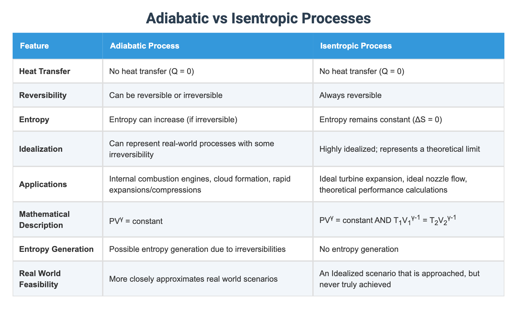
• An isentropic process is perfect: it's adiabatic ($Q=0$) AND reversible ($S_{gen}=0$). The result is $\Delta S=0$, or $s_2=s_1$.
• A real adiabatic process is still insulated ($Q=0$), but it is irreversible ($S_{gen}>0$). The result is $\Delta S>0$, or $s_2>s_1$.

The messiness of the real world actively creates entropy, even when no heat is being added or removed.

Let's look at this fantastic summary table which clearly separates these two ideas.

Visualizing the Benchmark: The h-s Diagram

This is where it all comes together. The enthalpy-entropy (h-s) diagram is the best tool to see exactly what irreversibilities do to the performance of a device.

Let's look at the two devices we analyzed last time: a turbine and a compressor.

Case 1: The Turbine (Getting Work Out)

Look at the diagram on the left.

1. The Ideal Path (1 → 2s): The fluid enters at State 1. In a perfect, isentropic turbine, the process is a straight vertical line down to State 2s (the 's' stands for isentropic). The work we get out is the drop in enthalpy: $w_{ideal}=h_1-h_{2s}$. This is the maximum possible work we can extract.
2. The Actual Path (1 → 2): In a real turbine, friction and turbulence generate entropy. So, as the enthalpy drops, the entropy increases. The path goes down and to the right, ending at State 2. The work we actually get out is $w_{actual}=h_1-h_2$.
3. The Result: Look closely at the diagram. The endpoint for the actual process, $h_2$, is higher on the enthalpy axis than the ideal endpoint, $h_{2s}$. This means the actual enthalpy drop is smaller. Therefore:
   $w_{actual}<w_{ideal}$
   We got less work out of our real turbine! The energy difference, $h_2-h_{2s}$, represents the work that was "lost" to friction and converted into useless additional heat in the exhaust fluid.

Case 2: The Compressor (Putting Work In)

Now look at the diagram on the right.

1. The Ideal Path (1 → 2s): The fluid enters at State 1. To compress it to a higher pressure, we need to put work in, raising its enthalpy. The ideal, isentropic path is a straight vertical line up to State 2s. The work we must put in is $w_{ideal}=h_{2s}-h_1$. This is the minimum possible work required.
2. The Actual Path (1 → 2): In a real compressor, friction and turbulence again generate entropy. So, as we increase the enthalpy, the entropy also increases. The path goes up and to the right, ending at State 2. The work we actually have to put in is $w_{actual}=h_2-h_1$.
3. The Result: The actual endpoint, $h_2$, is higher than the ideal endpoint, $h_{2s}$. This means the actual enthalpy increase is larger. Therefore:
   $w_{actual}>w_{ideal}$
   We had to put in more work to get the job done! The extra work, $w_{actual}-w_{ideal}$, was wasted overcoming friction and just made the outgoing fluid hotter than it needed to be for that final pressure. This is why your bicycle pump gets hot—a lot of your work is being wasted as friction, generating entropy and heat.

So, Why is the Isentropic Benchmark Useful?

We've established that real devices always underperform compared to the isentropic ideal. So why is this "perfect" calculation the first thing every engineer learns?

As the reading confirms, the isentropic process is the perfect benchmark for three main reasons:

1. It sets the theoretical limit. The isentropic calculation tells you the absolute best-case scenario. It answers the question, "What is the most work I can possibly get?" or "What is the least work I must put in?". This is vital for knowing if a proposed design is even feasible. If someone claims their new turbine design produces more work than the isentropic calculation allows, you know their claim violates the Second Law of Thermodynamics.

2. It provides a standard for comparison. Imagine two different companies sell compressors. Company A's compressor requires 300 kJ/kg of work. Company B's requires 320 kJ/kg. Which is better? You can't know without a benchmark. If you calculate the ideal isentropic work is 250 kJ/kg, you can now compare them fairly. You can say how "efficient" each one is relative to perfection.

3. It helps diagnose problems. If you have a large industrial gas compressor, you can measure its inlet and outlet temperatures and pressures. You can then calculate what the outlet temperature should be if the compressor were isentropic. If your actual outlet temperature is much, much higher than the ideal one, it's a huge red flag. It tells you that there's excessive entropy generation, likely due to problems like internal wear, leaks, or friction. The benchmark turns from a theoretical idea into a practical diagnostic tool.

Summary of Key Takeaways

Excellent work today. We've connected the dots between the ideal world of calculations and the messy, real world of machines.

• Real-world devices like turbines and compressors contain irreversibilities (friction, turbulence) that make them less than perfect.
• These irreversibilities generate entropy, causing the entropy of the fluid to increase as it passes through the device ($s_2>s_1$), even if the device is perfectly insulated (adiabatic).
• On an h-s diagram, the ideal isentropic process ($s=constant$) is a vertical line. The real-world process curves to the right (in the direction of increasing entropy).
• This deviation means a real turbine produces less work than the ideal, and a real compressor requires more work than the ideal.
• The isentropic process serves as the perfect benchmark or "gold standard" because it defines the theoretical maximum performance possible under the laws of thermodynamics, allowing us to compare and diagnose real machines.

Preview of the Next Lesson

We've spent this whole lesson talking about how real devices fall short of the ideal benchmark. The natural next question is, "How much do they fall short?"

In our next lesson, we will quantify this comparison by defining isentropic efficiency. We will create a simple ratio—a percentage—that tells us exactly how good our real turbine or compressor is compared to its perfect, isentropic counterpart. This will give us the single most important number for characterizing the performance of these real-world devices.