Using the First Derivative Test to Find Extrema

Hello! Welcome to our next lesson.

In our last session, we focused on using the sign of the first derivative, $f^{'} (x)$ , to determine the intervals where a function is increasing or decreasing. Today, we'll build directly on that knowledge to examine the specific points where the function changes direction. These "turning points" are the peaks and valleys of the graph, and they are crucial for understanding a function's behaviour.

By the end of this lesson, you will be able to find and classify these turning points as local (or relative) maxima and local (or relative) minima using a method called the First Derivative Test.

1. From Increasing/Decreasing to Extrema

Let's start with the logic, which flows directly from our last lesson. We know that the points where the gradient (slope) is zero, called stationary points or critical points, are where a function might change from increasing to decreasing, or vice versa.

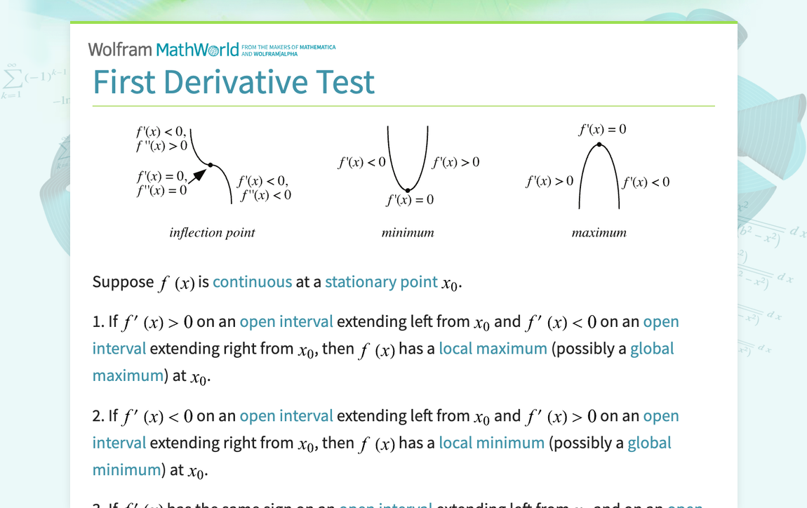
If a function is increasing ( $f^{'} (x) > 0$ ) and then switches to decreasing ( $f^{'} (x) < 0$ ), it must have reached a peak. This is a local maximum.
If a function is decreasing ( $f^{'} (x) < 0$ ) and then switches to increasing ( $f^{'} (x) > 0$ ), it must have bottomed out in a valley. This is a local minimum.
What if the sign doesn't change? If a function is increasing, flattens out, and then continues increasing, the stationary point is neither a maximum nor a minimum. This is often a point of inflection, which we'll explore more later.

The image below, from Wolfram MathWorld, provides a superb visual summary of this core concept.

First Derivative Test Illustration — This diagram illustrates the First Derivative Test. Notice how for a local minimum, the gradient f'(x) changes from negative to positive. For a local maximum, the gradient changes from positive to negative. At a point of inflection, the sign does not change.

2. The First Derivative Test: A Step-by-Step Guide

The First Derivative Test is a systematic procedure for finding and classifying these local extrema. It formalises the logic we just discussed.

Here is the process:

Find the derivative of the function, $f^{'} (x)$ .
Find the critical numbers. These are the candidates for our maxima and minima. They occur where:
- The derivative is zero: $f^{'} (x) = 0$ .
- The derivative is undefined (e.g., division by zero in the derivative's expression).
Create a sign table (or sign chart). Use the critical numbers you found to divide the number line into intervals.
Test each interval. Pick a convenient test number from within each interval and substitute it into the derivative, $f^{'} (x)$ , to find out if the gradient is positive (+) or negative (-) in that region.
Classify the critical points. Analyse the sign changes across each critical number:
- A change from + to - indicates a local maximum.
- A change from - to + indicates a local minimum.
- No sign change (e.g., + to + or - to -) means the point is not a local extremum.
Find the y-coordinates. To get the full coordinates of the maximum or minimum point, substitute the critical number (the x-value) back into the original function, $f (x)$ .

3. Worked Examples in Action

Seeing this process applied is the best way to learn it. Let's watch a couple of videos that walk through different types of problems.

Example 1: A Polynomial Function

First, let's see how this test works on a standard polynomial function, which will have multiple turning points.

Relative Extrema, Local Maximum and Minimum, First Derivative Test, Critical Points- Calculus

This video from The Organic Chemistry Tutor provides a clear, step-by-step example using a cubic function. This is a perfect illustration of the standard procedure.

Watch this segment from 05:27 to 08:32. Pay close attention to how he finds the two critical points by factorising (factoring) the derivative, creates a sign chart, and uses the sign changes to classify each point as a maximum or a minimum.

The process shown in the video is summarised perfectly in the following image. It shows the algebraic steps to find the critical points on the left and the sign table analysis on the right.

Finding and Classifying Stationary Points Using the First Derivative Test — This image shows the complete process for the function f(x) = x³ + 6x² - 15x + 3. The derivative is found, set to zero to find critical points x=-5 and x=1. The sign table then confirms that (-5, 103) is a local maximum and (1, -5) is a local minimum.

Example 2: A Function with an Undefined Derivative

It's important to remember that critical numbers can also occur where the derivative is undefined. This is common in functions with roots or fractional indices.

Calculus 1 Lecture 3.3: The First Derivative Test for Increasing and Decreasing

Professor Leonard works through an excellent example involving a fractional power, which leads to a derivative with a variable in the denominator. This highlights the importance of checking for undefined points.

Watch this example from 17:12 to 26:02. Notice how he finds critical numbers from both the numerator (where f'(x)=0) and the denominator (where f'(x) is undefined). He then uses both on his sign table to analyse the function's behaviour.

This second example completes the picture by showing that you must consider all types of critical points to fully analyse a function.

Test your understanding!

Find and classify the local extrema for the function $f (x) = 2 x^{3} + 3 x^{2} - 12 x$ .

Show answer

Find the derivative:
$f^{'} (x) = 6 x^{2} + 6 x - 12$
Find the critical numbers: Set $f^{'} (x) = 0$ .
$6 x^{2} + 6 x - 12 = 0$
$6 (x^{2} + x - 2) = 0$
$6 (x + 2) (x - 1) = 0$
The critical numbers are $x = - 2$ and $x = 1$ . The derivative is a polynomial, so it is never undefined.
Create a sign table: The intervals are $(- \infty, - 2)$ , $(- 2, 1)$ , and $(1, \infty)$ .

Interval	Test Value	Sign of $f^{'} (x) = 6 (x + 2) (x - 1)$	Behaviour of $f (x)$
$x < - 2$	$x = - 3$	$6 (- 1) (- 4) = +$	Increasing
$- 2 < x < 1$	$x = 0$	$6 (2) (- 1) = -$	Decreasing
$x > 1$	$x = 2$	$6 (4) (1) = +$	Increasing

Classify the critical points:
- At $x = - 2$ , the sign changes from + to -, so this is a local maximum.
- At $x = 1$ , the sign changes from - to +, so this is a local minimum.
Find the y-coordinates:
- Maximum point: $f (- 2) = 2 (- 2)^{3} + 3 (- 2)^{2} - 12 (- 2) = - 16 + 12 + 24 = 20$ . The local maximum is at (-2, 20).
- Minimum point: $f (1) = 2 (1)^{3} + 3 (1)^{2} - 12 (1) = 2 + 3 - 12 = - 7$ . The local minimum is at (1, -7).

4. Formal Definitions and Summary

To consolidate your understanding, let's turn to a text-based resource that uses the British terminology you're familiar with.

Cambridge (CIE) A Level Maths Revision Notes

This revision note from Save My Exams provides a concise summary. It clearly defines stationary and turning points and lays out the first derivative test (which it calls 'Method A').

Please read the sections titled 'What are stationary points?' and the details under 'Method A: Compare the signs of the first derivative...'. The flowchart in this section is an excellent visual summary of the decision-making process.

Conclusion

You have now learned one of the most powerful applications of the first derivative: locating and classifying the peaks and valleys of a function. This is a fundamental skill for sketching graphs and solving optimisation problems.

Key Takeaways:

Local extrema (maxima and minima) occur at critical points, where the derivative is either zero or undefined.
The First Derivative Test is a systematic process for classifying these points by checking the sign of the derivative on either side.
A sign change from positive to negative ( $+$ to $-$ ) at a critical point indicates a local maximum.
A sign change from negative to positive ( $-$ to $+$ ) at a critical point indicates a local minimum.
To find the full coordinates of an extremum, substitute the x-value back into the original function, $f (x)$ .

In our next lesson, we will introduce the second derivative. This will give us information about a function's concavity—whether the graph is curved upwards or downwards—and provide us with an alternative method for classifying stationary points called the Second Derivative Test.

Recommended resources