Concavity and Inflection Points

1. What is Concavity?

While the first derivative tells us if a function is going up or down, the second derivative tells us how it's curving as it does so.

Imagine driving along the curve of a graph.

• If you are turning your steering wheel to the left, the curve is bending upwards.
• If you are turning your steering wheel to the right, the curve is bending downwards.

This "bending" is called concavity.

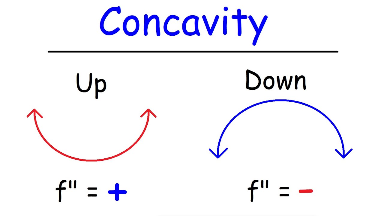
Terminology and The Second Derivative

There are two types of concavity, and it's important to clarify the terminology, as it can differ.

• Concave Down: The graph is bending downwards, like a frown or the letter 'n'. The tangents to the curve lie above the graph. In this region, the gradient, $f^{\prime }(x)$, is decreasing. Since the gradient is decreasing, its derivative, which is the second derivative $f^{\prime \prime }(x)$, must be negative.
  $f^{\prime \prime }(x)<0⟹\text{Concave Down}$

• Convex (or Concave Up): The graph is bending upwards, like a smile or the letter 'u'. The tangents to the curve lie below the graph. Here, the gradient, $f^{\prime }(x)$, is increasing. Therefore, the second derivative, $f^{\prime \prime }(x)$, must be positive.
  $f^{\prime \prime }(x)>0⟹\text{Convex (Concave Up)}$

Your school background likely used the term convex, and we will primarily use that term. I will include the American equivalent, "concave up," in brackets for your reference.

To see these definitions explained, please watch the short introductory segment of this video.

2. Finding Intervals of Concavity

The process for finding the intervals where a function is convex or concave down is very similar to the First Derivative Test you used in the last lesson. The only difference is that we now apply it to the second derivative.

Procedure:

1. Given a function $f(x)$, find its second derivative, $f^{\prime \prime }(x)$.
2. Find the values of $x$ where $f^{\prime \prime }(x)=0$ or where $f^{\prime \prime }(x)$ is undefined. These values are the boundaries of our intervals.
3. Create a sign table for $f^{\prime \prime }(x)$ using these boundary points.
4. Choose a test value from each interval and substitute it into $f^{\prime \prime }(x)$ to determine its sign (+ or -).
5. Interpret the results:
   • If $f^{\prime \prime }(x)>0$, the function is convex on that interval.
   • If $f^{\prime \prime }(x)<0$, the function is concave down on that interval.

Let's see this procedure in action.

3. Points of Inflection

A point of inflection is a point on the graph where the concavity changes. This is where the curve switches from convex to concave down, or vice versa.

For a point of inflection to exist at $x=c$, two conditions must be met:

1. The second derivative at that point is zero or undefined ($f^{\prime \prime }(c)=0$ or is undefined).
2. The sign of the second derivative $f^{\prime \prime }(x)$ changes as we move across $x=c$.

The second condition is crucial. Just because $f^{\prime \prime }(c)=0$ does not automatically guarantee a point of inflection. We must test the sign of $f^{\prime \prime }(x)$ on either side to be sure. This is often called a "neighbourhood test."

This resource from the University of Sydney summarises it perfectly. Under the heading 'Points of inflection', it states: "A point of inflection occurs at a point where d²y/dx² = 0 AND there is a change in concavity of the curve at that point."

The following video explains why this test is so important.

4. A Step-by-Step Guide to Finding Points of Inflection

Let's combine everything into a single procedure.

Procedure:

1. Find the second derivative, $f^{\prime \prime }(x)$.
2. Find the x-coordinates of all potential points of inflection by solving $f^{\prime \prime }(x)=0$.
3. For each potential point $x=c$, check the sign of $f^{\prime \prime }(x)$ on either side (e.g., at $c-h$ and $c+h$ for some small $h$).
4. If the sign of $f^{\prime \prime }(x)$ changes, then there is a point of inflection at $x=c$.
5. To find the full coordinates of the point, substitute $x=c$ back into the original function, $f(x)$.

Let's watch one final example that ties this all together.

Conclusion

You've now added another powerful tool to your calculus toolbox. By using the second derivative, you can determine the curvature of a function, which is essential for creating accurate graph sketches and understanding a function's behaviour in more detail.

Key Takeaways:

• The second derivative, $f^{\prime \prime }(x)$, describes a function's concavity.
• If $f^{\prime \prime }(x)>0$, the function is convex (concave up).
• If $f^{\prime \prime }(x)<0$, the function is concave down.
• A point of inflection is a point where the concavity changes.
• To find points of inflection, you must find where $f^{\prime \prime }(x)=0$ and then confirm that the sign of $f^{\prime \prime }(x)$ changes around that point.

In our next lesson, we will see another use for the second derivative. It can be used as an alternative to the First Derivative Test for classifying stationary points as local maxima or minima. This method, called the Second Derivative Test, is often a very quick and efficient shortcut.