The Second Derivative Test

1. The Intuition: Concavity at a Stationary Point

Let's start with the core idea, which builds directly on what you learned about concavity. Imagine you've found a stationary point on a graph. You know the tangent line at this point is horizontal. Now, consider the shape of the curve at that exact spot:

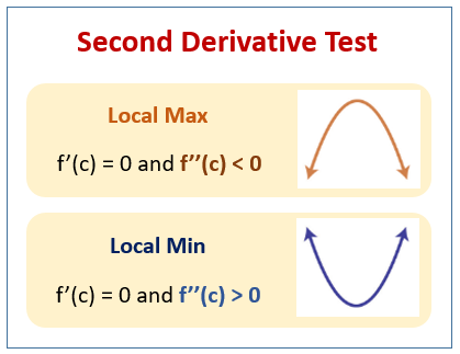
• If the function is convex (concave up) at the stationary point, the curve looks like a 'U'. A horizontal tangent on a 'U' shape can only happen at the very bottom. Therefore, the point must be a local minimum.
• If the function is concave down at the stationary point, the curve looks like an inverted 'U'. A horizontal tangent on this shape can only occur at the very top. Therefore, the point must be a local maximum.

This simple connection between the curve's shape and the type of stationary point is the foundation of the Second Derivative Test.

The following video from Khan Academy provides an excellent visual explanation of this intuition.

This relationship is summarised perfectly in the image below.

2. The Formal Second Derivative Test

Now, let's translate this intuition into a formal mathematical procedure. As you know from the previous lesson, the sign of the second derivative, $f^{\prime \prime }(x)$, tells us the concavity. We can use this to create a formal test.

To summarise the rules for a function $f(x)$ at a stationary point $x=c$ (where $f^{\prime }(c)=0$):

1. If $f^{\prime \prime }(c)>0$, the function is convex at $c$, so $f$ has a local minimum at $x=c$.
2. If $f^{\prime \prime }(c)<0$, the function is concave down at $c$, so $f$ has a local maximum at $x=c$.
3. If $f^{\prime \prime }(c)=0$, the test is inconclusive. It tells us nothing, and we must use a different method.

3. Applying the Test: A Worked Example

Let's see the test in action. The process involves finding the stationary points first, then using the second derivative to classify them.

1. Find the first derivative, $f^{\prime }(x)$.
2. Solve $f^{\prime }(x)=0$ to find the x-coordinates of the stationary points.
3. Find the second derivative, $f^{\prime \prime }(x)$.
4. For each stationary point $x=c$, calculate the value of $f^{\prime \prime }(c)$.
5. Apply the rules of the Second Derivative Test to classify each point.

The following video demonstrates this process clearly. The presenter has already found the stationary points in a previous part of the video; here, we focus on how he uses the second derivative to classify them.

4. The Inconclusive Case: When $f^{\prime \prime }(c)=0$

The third rule of the test is very important: if the second derivative is zero at a stationary point, the test fails. It doesn't mean there isn't a maximum or minimum, only that this specific test cannot determine it. The point could be a local maximum, a local minimum, or a point of inflection.

So, what do you do when the test is inconclusive?

You must revert to the First Derivative Test. That is, you test the sign of the first derivative, $f^{\prime }(x)$, on either side of the stationary point to see if the gradient changes from positive to negative (local max), negative to positive (local min), or stays the same (point of inflection).

Let's walk through an example of this from the resource The Second Derivative Test - Differential Calculus. Consider the function $f(x)=3x^5-5x^3+3$.

1. First Derivative: $f^{\prime }(x)=15x^4-15x^2$
2. Stationary Points: $15x^2(x^2-1)=0$, so $x=-1,0,1$.
3. Second Derivative: $f^{\prime \prime }(x)=60x^3-30x$

Now, let's test the points:

• $f^{\prime \prime }(-1)=-60+30=-30<0⟹$ Local Maximum at $x=-1$.
• $f^{\prime \prime }(1)=60-30=30>0⟹$ Local Minimum at $x=1$.
• $f^{\prime \prime }(0)=0-0=0⟹$ Test is Inconclusive.

We must use the First Derivative Test for $x=0$. We need to check the sign of $f^{\prime }(x)=15x^2(x^2-1)$ in the neighbourhood of $x=0$.

• To the left of 0 (e.g., at $x=-0.5$): $f^{\prime }(-0.5)=15(-0.5{)}^2((-0.5{)}^2-1)=15(0.25)(0.25-1)=(+)(-)=\text{negative}$.
• To the right of 0 (e.g., at $x=0.5$): $f^{\prime }(0.5)=15(0.5{)}^2((0.5{)}^2-1)=15(0.25)(0.25-1)=(+)(-)=\text{negative}$.

Since the gradient is negative on both sides of $x=0$, the function is decreasing, flattens out, and then continues decreasing. Therefore, the point at $x=0$ is neither a maximum nor a minimum; it is a stationary point of inflection.

Conclusion

You've now learned a valuable shortcut for classifying stationary points. While the First Derivative Test always works, the Second Derivative Test is often quicker when the second derivative is easy to compute and non-zero.

Key Takeaways:

• The Second Derivative Test classifies a stationary point $x=c$ based on the sign of $f^{\prime \prime }(c)$.
• Local Minimum: If $f^{\prime }(c)=0$ and $f^{\prime \prime }(c)>0$ (convex/concave up).
• Local Maximum: If $f^{\prime }(c)=0$ and $f^{\prime \prime }(c)<0$ (concave down).
• Inconclusive: If $f^{\prime }(c)=0$ and $f^{\prime \prime }(c)=0$. In this case, you must use the First Derivative Test to classify the point.

In our next lesson, we will begin applying these powerful tools—finding and classifying extrema—to solve practical optimisation (optimization) problems, where the goal is to find the maximum or minimum value of something, like profit, cost, or area.