Absolute Extrema in Optimization

1. Absolute vs. Relative Extrema: A Quick Recap

Before we dive in, let's clarify the difference between the local extrema you've been working with and the absolute extrema we need for optimisation.

• Relative (or Local) Extrema: These are the 'hills' and 'valleys' in a function. A point is a relative maximum if it's higher than all the points immediately surrounding it.
• Absolute Extrema: This is the single highest or lowest point a function reaches over its entire domain (or a specified interval).

In optimisation, we are almost always looking for the absolute maximum or minimum.

2. A Strategy for Solving Optimisation Problems

Optimisation problems can seem tricky at first because they are often presented as word problems. The key is to translate the words into mathematics. The calculus part is usually straightforward; the setup is the most important part.

Here is a systematic approach that we will use throughout this lesson.

Let's summarise that strategy:

1. Understand the Goal: Identify what quantity you need to maximise or minimise. Draw a picture and label variables.
2. Write the Equations:
   • Objective Function: This is the function you want to optimise (e.g., Area = $L\times W$).
   • Constraint Equation: This is the restriction or condition you're given (e.g., Perimeter = 100m).
3. Create a Single-Variable Function: Use the constraint equation to substitute one variable into the objective function. This leaves you with a function of just one variable (e.g., $A(x)$). Determine the domain of this function—the set of all possible, realistic values for your variable.
4. Find the Critical Points: Take the derivative of your single-variable function and set it to zero to find the critical points.
5. Test and Verify: This is where we find the absolute extremum.
   • If the domain is a closed interval [a, b]: Evaluate the function at the critical points and at the endpoints (a and b). The largest value is the absolute maximum, and the smallest is the absolute minimum.
   • If the domain is an open interval: If there is only one critical point, you can use the First or Second Derivative Test to confirm if it's a maximum or minimum. If it is, it must be the absolute extremum.
6. State the Answer: Make sure you answer the original question. Do you need to provide dimensions, cost, or the maximised value itself?

3. Example 1: Maximising Area with a Fixed Perimeter

This is a classic optimisation problem. Let's watch an excellent, detailed walkthrough that puts our strategy into practice.

Notice how Professor Leonard followed the strategy perfectly:

• Goal: Maximise Area, $A=xy$.
• Constraint: Perimeter is 100 ft, so $2x+2y=100$.
• Single Variable: Solved the constraint for $y$ to get $A(x)=x(50-x)$. He also identified the domain for $x$ was the closed interval $[0,50]$.
• Critical Points: Found $A^{\prime }(x)=0$ when $x=25$.
• Test: He checked the value of the Area function at the critical point ($x=25$) and the endpoints ($x=0$ and $x=50$).
  • $A(0)=0$
  • $A(50)=0$
  • $A(25)=625$
• Answer: The maximum area of 625 sq ft occurs when the dimensions are 25 ft by 25 ft.

This method of testing the critical points and the endpoints is the standard procedure for finding absolute extrema on a closed interval.

4. Example 2: Maximising the Volume of a Box

Let's try another common problem type: creating an open-topped box from a flat sheet of cardboard by cutting squares from the corners.

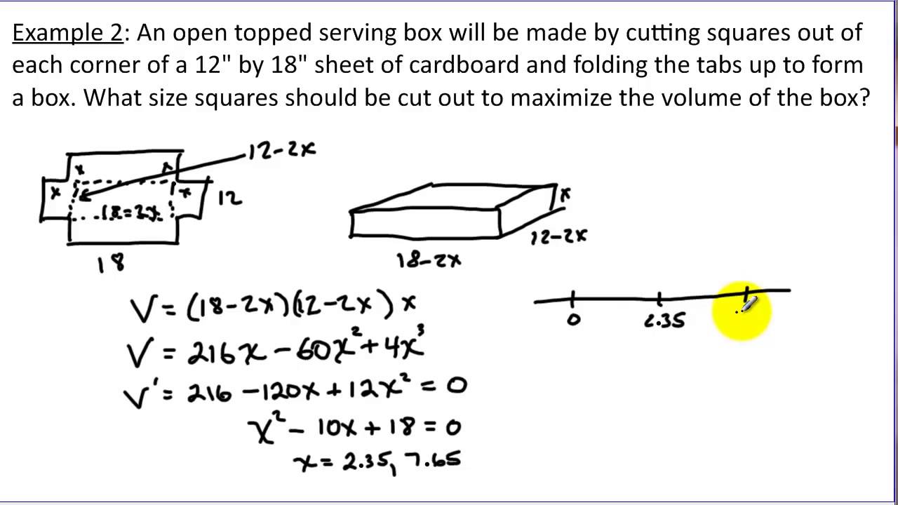
Let's work through this problem using a text-based resource.

5. Optimisation on Open Intervals

In the box problem, the domain for $x$ was technically an open interval, like $(0,12)$ in the example. What happens when the domain is not a closed interval, and we don't have endpoints to test?

This is where the derivative tests come back into play. If a function is continuous on an open interval and has only one critical point, then:

• If that point is a local minimum, it must also be the absolute minimum.
• If that point is a local maximum, it must also be the absolute maximum.

We can confirm if it's a local minimum or maximum using the Second Derivative Test, which you learned in the previous lesson. Let's see this in action.

Example 3: Minimising the Surface Area of a Can

Imagine you are designing a cylindrical can. The can must hold a specific volume (say, 1000 cm³), and you want to use the least amount of metal to build it. This means you want to minimise the surface area for a fixed volume.

• Objective (Minimise): Surface Area, $S$. For a cylinder with radius $r$ and height $h$, $S=2\pi r^2+2\pi rh$ (the area of the top and bottom circles plus the area of the side).
• Constraint (Fixed): Volume, $V=\pi r^{2}h=1000$.

We can use the constraint to find $h$ in terms of $r$: $h=\frac{1000}{\pi r^2}$.
Now, substitute this into the surface area formula to get a function of one variable, $r$:
$S(r)=2\pi r^2+2\pi r\left(\frac{1000}{\pi r^2}\right)=2\pi r^2+\frac{2000}{r}$
The domain for the radius $r$ is $(0,\infty )$, which is an open interval. Now, we find the critical point and use the second derivative test to prove it's a minimum.

As he showed, after finding the critical value for $r$, he calculated the second derivative $S^{\prime \prime }(r)$. Since $S^{\prime \prime }(r)$ was positive at the critical point, it confirmed the function was convex (concave up), proving he had found a local minimum. And because it was the only critical point on the open interval, it had to be the absolute minimum.

Conclusion

You have now learned the complete process for tackling optimisation problems, one of the most practical applications of differential calculus. The method may seem long, but it is systematic and powerful.

Key Takeaways:

• Optimisation is about finding the absolute maximum or minimum of a quantity.
• The first step is always to define your objective function (what you're optimising) and your constraint equation (the limitation).
• Use the constraint to rewrite the objective function in terms of a single variable.
• Find the critical points by setting the first derivative to zero.
• If the domain is a closed interval, test the function's value at the critical points and the endpoints.
• If the domain is an open interval with only one critical point, use the Second Derivative Test to verify if it is a maximum or minimum.

In our next lesson, we will explore another application of derivatives called L'Hôpital's Rule, which provides a clever way to evaluate certain types of limits that would otherwise be difficult to solve.