Graphing Polynomials: A Synthesis Approach

1. The Method: A Step-by-Step Guide to Sketching Polynomials

Sketching a polynomial is like solving a puzzle. We have several clues (the key features), and our task is to assemble them into a single, coherent picture. Here is a systematic process you can follow every time.

A 5-Step Process for Graphing a Polynomial

1. Find the y-intercept: This is the point where the graph crosses the y-axis. You can find it by calculating $f(0)$ (i.e., substituting $x=0$ into the function).
2. Find the x-intercepts (Roots): These are the points where the graph crosses or touches the x-axis. For a polynomial in factorised form, you can find them by setting each factor to zero and solving for $x$.
3. Analyse the Multiplicity of the Roots: Look at the power (exponent) of each factor.
   • Odd multiplicity (1, 3, 5, ...): The graph crosses the x-axis at this root.
   • Even multiplicity (2, 4, 6, ...): The graph touches the x-axis at this root and "bounces" back.
4. Determine the End Behaviour: Use the Leading Term Test from our previous lesson.
   • Find the degree ($n$) of the polynomial by summing the multiplicities of the roots.
   • Find the sign of the leading coefficient ($a_n$).
   • Use the degree (even/odd) and sign (positive/negative) to determine if the graph rises or falls on the far left and far right.
5. Sketch the Graph:
   • Mark the intercepts on your axes.
   • Start drawing from the far left, following the end behaviour.
   • Connect the intercepts, making sure the graph crosses or bounces correctly according to the multiplicity of each root.
   • Ensure the finished sketch is a smooth curve that matches the end behaviour on the right and does not have more than $n-1$ turning points.

The following resource provides a detailed walkthrough of this process with excellent examples. It uses the American term "zeros" for "roots", but the method is identical.

2. Seeing it in Action: Video Walkthroughs

Now that you have the step-by-step process, let's watch it being applied. These videos will help solidify your understanding, especially regarding the behaviour at the roots.

This first video uses British terminology and provides a quick, clear introduction to sketching polynomials that are already factorised.

The BareauMaths video did an excellent job showing what happens for multiplicities of 1 (cross) and 2 (bounce). What happens for higher multiplicities? The next video elaborates on this.

Key Distinction in Multiplicity:

• Multiplicity 1: Crosses the x-axis (like a line).
• Multiplicity 2: Touches the x-axis and bounces off (like a parabola's vertex).
• Multiplicity 3: Crosses the x-axis, but flattens horizontally as it passes through (like the graph of $y=x^3$ at the origin).

3. Let's Sketch One Together

Let's apply the 5-step process to a new function: $f(x)=(x-1{)}^2(x+3)$.

1. Find the y-intercept:

   • Set $x=0$: $f(0)=(0-1{)}^2(0+3)=(-1{)}^2(3)=1\times 3=3$.
   • The y-intercept is at $(0,3)$.

2. Find the x-intercepts (Roots):

   • Set each factor to zero:
     • $(x-1{)}^2=0⟹x-1=0⟹x=1$
     • $x+3=0⟹x=-3$
   • The roots are at $x=1$ and $x=-3$.

3. Analyse the Multiplicity:

   • For the root $x=1$, the factor is $(x-1{)}^2$. The multiplicity is 2 (even), so the graph will touch and bounce at $x=1$.
   • For the root $x=-3$, the factor is $(x+3{)}^1$. The multiplicity is 1 (odd), so the graph will cross at $x=-3$.

4. Determine the End Behaviour:

   • Degree: The degree is the sum of the multiplicities: $2+1=3$. This is an odd degree polynomial.
   • Leading Coefficient: Imagine expanding the expression: $(x-1{)}^2(x+3)=(x^2-2x+1)(x+3)$. The leading term would be $x^2\times x=x^3$. The coefficient is $+1$, which is positive.
   • Conclusion: For an odd degree, positive leading coefficient polynomial, the end behaviour is Falls Left, Rises Right.

5. Sketch the Graph:

   • Plot the intercepts: $(0,3)$, $(-3,0)$, and $(1,0)$.
   • Start from the far left (falling).
   • The graph rises to the first root at $x=-3$ and crosses it.
   • The graph continues to rise, passing through the y-intercept at $(0,3)$.
   • It must turn around to come back down to the next root at $x=1$.
   • At $x=1$, the graph touches the axis and bounces off, heading back up.
   • This upward movement matches our "Rises Right" end behaviour.

Here is what the final sketch should look like. Notice it has two turning points, which is the maximum for a degree 3 polynomial ($n-1=3-1=2$).

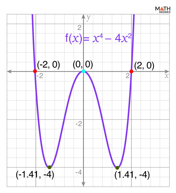
(Correction: A better image representing the specific function $f(x)=(x-1{)}^2(x+3)$ would show the bounce at x=1 and the crossing at x=-3. Imagine a curve that does exactly that, passing through y=3.)

Conclusion

Today we have successfully combined all our analytical tools to build a complete picture of a polynomial function. By following a structured process, you can confidently translate a polynomial's equation into a visual sketch that captures its most important characteristics.

Key Takeaways:

• A reliable 5-step process for sketching polynomials involves finding intercepts, analysing multiplicities, determining end behaviour, and then connecting the points with a smooth curve.
• The multiplicity of a root is your guide for how the graph behaves at the x-axis: odd multiplicity means it crosses, while even multiplicity means it touches and bounces.
• The end behaviour provides the "frame" for your sketch, telling you where the graph starts and ends.
• The number of turning points (at most $n-1$) serves as a final check on your sketch's shape.

Preview of the Next Lesson:
We have developed a strong understanding of polynomial functions. Next, we will venture into a related family of functions: rational functions. These are functions formed by dividing one polynomial by another, like $f(x)=\frac{x+1}{x-2}$. This fractional nature introduces fascinating new graphical features called asymptotes—lines that the graph approaches but never touches. We will learn how to find and analyse these to sketch rational functions.