Polynomial End Behavior and Turning Points

1. End Behaviour: The Leading Term Test

The end behaviour of a function describes what happens to its y-values as the x-values become extremely large in either the positive ($x\to \infty$) or negative ($x\to -\infty$) direction. For polynomials, the end behaviour is determined entirely by the term with the highest power of $x$, known as the leading term. As $x$ gets very large, the influence of this single term outweighs all others combined.

To determine the end behaviour, we need to examine two features of the leading term, $a_n{x}^n$:

1. The degree ($n$): Whether it is even or odd.
2. The sign of the leading coefficient ($a_n$): Whether it is positive or negative.

This gives us four possible combinations, which can be summarised as the Leading Term Test.

The following video provides an excellent explanation of this concept and how it relates to the simple power functions you are already familiar with (like $y=x^2$ and $y=x^3$).

As the video explained, these four scenarios determine if the graph rises or falls on the left and right sides. This chart provides a fantastic visual summary:

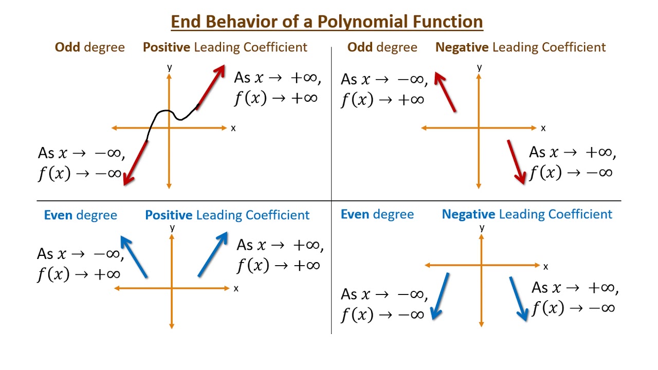
Another way to describe this, which you may see in some texts, is by referencing quadrants. For example, a polynomial with an odd degree and a positive leading coefficient (like $y=x^3$) "extends from Quadrant 3 to Quadrant 1".

2. Turning Points: The Hills and Valleys

Now that we know what happens at the ends of the graph, let's consider what happens in the middle. The smooth, flowing curves of polynomial graphs have peaks and valleys where they change direction. These are called turning points.

• A turning point where the function changes from increasing to decreasing is a local maximum.
• A turning point where the function changes from decreasing to increasing is a local minimum.

There is a simple and direct relationship between the degree of a polynomial and the number of turning points it can have.

As the resource stated, the key rule is:

A polynomial of degree $n$ has at most $n-1$ turning points.

This is a powerful piece of information. A cubic function (degree 3) can have at most $3-1=2$ turning points. A quintic function (degree 5) can have at most $5-1=4$ turning points. It can have fewer, but never more.

To dive a little deeper, let's explore how the parity (evenness or oddness) of the degree affects the number of turning points.

This parity rule makes sense when you combine it with end behaviour. An even-degree polynomial must start and end going in the same direction (e.g., up and up), so to connect the ends it must change direction an odd number of times. Conversely, an odd-degree polynomial must start and end in opposite directions, requiring an even number of turns.

3. A Quick Look at Behaviour at the Roots: Multiplicity

Finally, let's connect today's topic back to our previous lesson on finding roots. In the last exercise, you found that the polynomial $P(x)=(x+2)(x-3{)}^2$ had a "repeated root" at $x=3$. The exponent on the factor, in this case 2, is called the multiplicity of the root. This number tells us how the graph behaves when it meets the x-axis at that root.

• Odd Multiplicity (e.g., 1, 3, 5...): The graph crosses the x-axis at the root.
• Even Multiplicity (e.g., 2, 4, 6...): The graph touches the x-axis and "bounces" off, returning in the direction it came from.

This concept is explained in the first part of the Professor Leonard video. While not strictly required by today's learning outcome, it is essential for the next step of sketching graphs, so it's useful to see it now.

Conclusion

In this lesson, we have added two major tools to our polynomial analysis toolkit. By combining them with what we already know about roots, we can now predict the overall shape of a polynomial's graph from its equation alone.

Key Takeaways:

• End Behaviour is determined by the leading term. We look at the degree (even/odd) and the leading coefficient's sign (positive/negative) to know if the graph rises or falls on the far left and right.
• Turning Points are the local maxima and minima where the graph changes direction. A polynomial of degree $n$ has at most $n-1$ turning points.
• The number of turning points has the opposite parity to the degree: odd degree functions have an even number of turning points, and even degree functions have an odd number.

Preview of the Next Lesson:
We have all the pieces now: roots (x-intercepts), y-intercept, end behaviour, and turning points. In our next lesson, we will sketch the graph of a polynomial function by synthesising (synthesizing) its key features. We will take a polynomial equation from start to finish and produce a detailed sketch of its graph.