Analyzing Rational Functions

1. What is a Rational Function?

A rational function is any function that can be written as the ratio of two polynomials, $f(x)=\frac{P(x)}{Q(x)}$, where $Q(x)$ is not the zero polynomial.

Examples include:

• $f(x)=\frac{1}{x}$
• $g(x)=\frac{x+3}{x^2-9}$
• $h(x)=\frac{2x^2-x+1}{x-2}$

The most important new characteristic of rational functions comes from the denominator. Since division by zero is undefined, we must pay special attention to any x-values that make the denominator, $Q(x)$, equal to zero. These values are not in the function's domain and they create discontinuities in the graph.

Watch this brief introduction to get a feel for what these functions and their discontinuities look like.

2. The First Step: Factorise and Find Restrictions

Just as with polynomials, our first step in analysing a rational function is to factorise (factor) the numerator and the denominator completely. This single step is the key that unlocks almost all of the function's secrets.

Once factorised, we can easily see the restrictions on the variable—the x-values that make the denominator zero. These are the locations of our discontinuities.

3. Types of Discontinuities: Vertical Asymptotes and Holes

The restrictions we just found tell us where the graph has breaks, but not what kind of breaks they are. There are two main types:

1. Vertical Asymptotes (Infinite Discontinuities): These are vertical lines that the graph approaches but never touches or crosses. A vertical asymptote occurs at $x=c$ if the factor $(x-c)$ remains in the denominator after we have simplified the function by cancelling any common factors. This corresponds to a "non-zero divided by zero" situation.

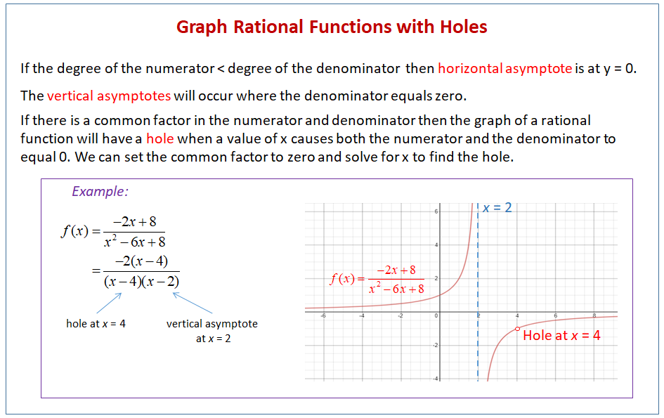
2. Holes (Removable Discontinuities): These are single points missing from the graph. A hole occurs at $x=c$ if the factor $(x-c)$ is a common factor in both the numerator and the denominator, and it gets cancelled out during simplification. This corresponds to a "zero divided by zero" situation.

The following text provides a formal definition and method for telling them apart.

To see this distinction in action, let's return to the JensenMath video, which has excellent examples of both scenarios.

Here is a visual summary of finding a hole:

4. End Behaviour: Horizontal and Slant Asymptotes

Next, we need to understand the function's end behaviour: what happens to the graph as $x$ approaches positive or negative infinity ($x\to \pm \infty$)? For polynomials, the graph would rise or fall forever. For rational functions, the graph will often level off and approach a horizontal or slanting line called a horizontal asymptote or slant (oblique) asymptote.

You can determine which type of asymptote exists by comparing the degree of the numerator ($N$) to the degree of the denominator ($D$).

The LibreTexts resource you looked at earlier has a fantastic summary of the three possible cases.

Here is a summary of the rules:

• Case 1: $N<D$ (Bottom-heavy)
  • The horizontal asymptote is the line $y=0$ (the x-axis).
• Case 2: $N=D$ (Equal degrees)
  • The horizontal asymptote is the line $y=\frac{a_n}{b_m}$, where $a_n$ and $b_m$ are the leading coefficients of the numerator and denominator, respectively.
• Case 3: $N=D+1$ (Top-heavy by one)
  • There is a slant (oblique) asymptote. You find its equation by performing polynomial division. The asymptote is the line defined by the quotient (you can ignore the remainder).

The following video segments show worked examples for each of these cases.

5. Finding the Intercepts

The final pieces of our analysis are the intercepts. This process is very similar to what we did with polynomials.

• y-intercept: To find where the graph crosses the y-axis, we evaluate the function at $x=0$. Simply calculate $f(0)$. If the function is undefined at $x=0$ (i.e., it's a vertical asymptote), there is no y-intercept.
• x-intercepts (Roots): To find where the graph crosses the x-axis, we set the function equal to zero and solve for $x$. A fraction $\frac{P(x)}{Q(x)}$ is equal to zero only when its numerator is zero. So, we set the numerator of the simplified function equal to zero to find the roots.

6. Putting It All Together: A Complete Analysis

Let's synthesise everything we've learned by analysing one function from start to finish.

Function: $F(x)=\frac{x^2-3x-28}{x^2-6x-40}$

Our Step-by-Step Analysis:

1. Factorise:

   • Numerator: $x^2-3x-28=(x-7)(x+4)$
   • Denominator: $x^2-6x-40=(x-10)(x+4)$
   • So, $F(x)=\frac{(x-7)(x+4)}{(x-10)(x+4)}$

2. Discontinuities:

   • The factor $(x+4)$ cancels out, so there is a hole at $x=-4$.
     • To find the y-coordinate, use the simplified function $g(x)=\frac{x-7}{x-10}$.
     • $g(-4)=\frac{-4-7}{-4-10}=\frac{-11}{-14}=\frac{11}{14}$.
     • The hole is at $(-4,\frac{11}{14})$.
   • The factor $(x-10)$ remains in the denominator, so there is a vertical asymptote at $x=10$.

3. End Behaviour Asymptote:

   • The degree of the numerator ($N=2$) is equal to the degree of the denominator ($D=2$).
   • This is Case 2. The horizontal asymptote is the ratio of the leading coefficients: $y=\frac{1}{1}=1$.
   • There is a horizontal asymptote at $y=1$.

4. Intercepts:

   • y-intercept: Find $F(0)$.
     • $F(0)=\frac{0^2-3(0)-28}{0^2-6(0)-40}=\frac{-28}{-40}=\frac{7}{10}$.
     • The y-intercept is at $(0,\frac{7}{10})$.
   • x-intercept (root): Set the simplified numerator to zero.
     • $x-7=0⟹x=7$.
     • The x-intercept is at $(7,0)$.

We have now successfully identified every key feature of the function, as summarised in the image.

Conclusion

In this lesson, we have developed a complete toolkit for analysing rational functions. By breaking down the function into its constituent parts, we can systematically uncover all the information needed to understand its behaviour.

Key Takeaways:

• Factorise First: Always start by factoring the numerator and denominator. This reveals the potential discontinuities.
• Discontinuities:
  • Vertical Asymptotes come from factors that remain in the denominator after simplification.
  • Holes come from factors that are cancelled out from the numerator and denominator.
• End Behaviour Asymptotes: The relationship between the degrees of the numerator ($N$) and denominator ($D$) determines the end behaviour.
  • $N<D⟹$ HA at $y=0$.
  • $N=D⟹$ HA at the ratio of leading coefficients.
  • $N=D+1⟹$ Slant asymptote found by division.
• Intercepts:
  • y-intercept: Find $f(0)$.
  • x-intercepts (Roots): Find the roots of the simplified numerator.

Preview of the Next Lesson:
We have successfully completed the "analysis" phase. We know how to find the entire "skeleton" of a rational function. In our next lesson, we will put these pieces together to achieve our next learning outcome: Sketch the graph of a rational function using its key features.