Hello! In our last lesson, we established the formal definition of the derivative as the limit of a difference quotient. You saw how to use this "first principles" method to find the derivative of functions like .
Today, we're going to breathe life into that abstract limit. Our goal is to interpret the derivative as the gradient (slope) of a tangent line and as an instantaneous rate of change. This is a crucial step, as it connects the algebraic process you learned to its powerful geometric and physical meanings. Understanding these interpretations is key to seeing why calculus is such a fundamental tool in science, technology, and beyond.
1. The Geometric Interpretation: Gradient of a Tangent Line
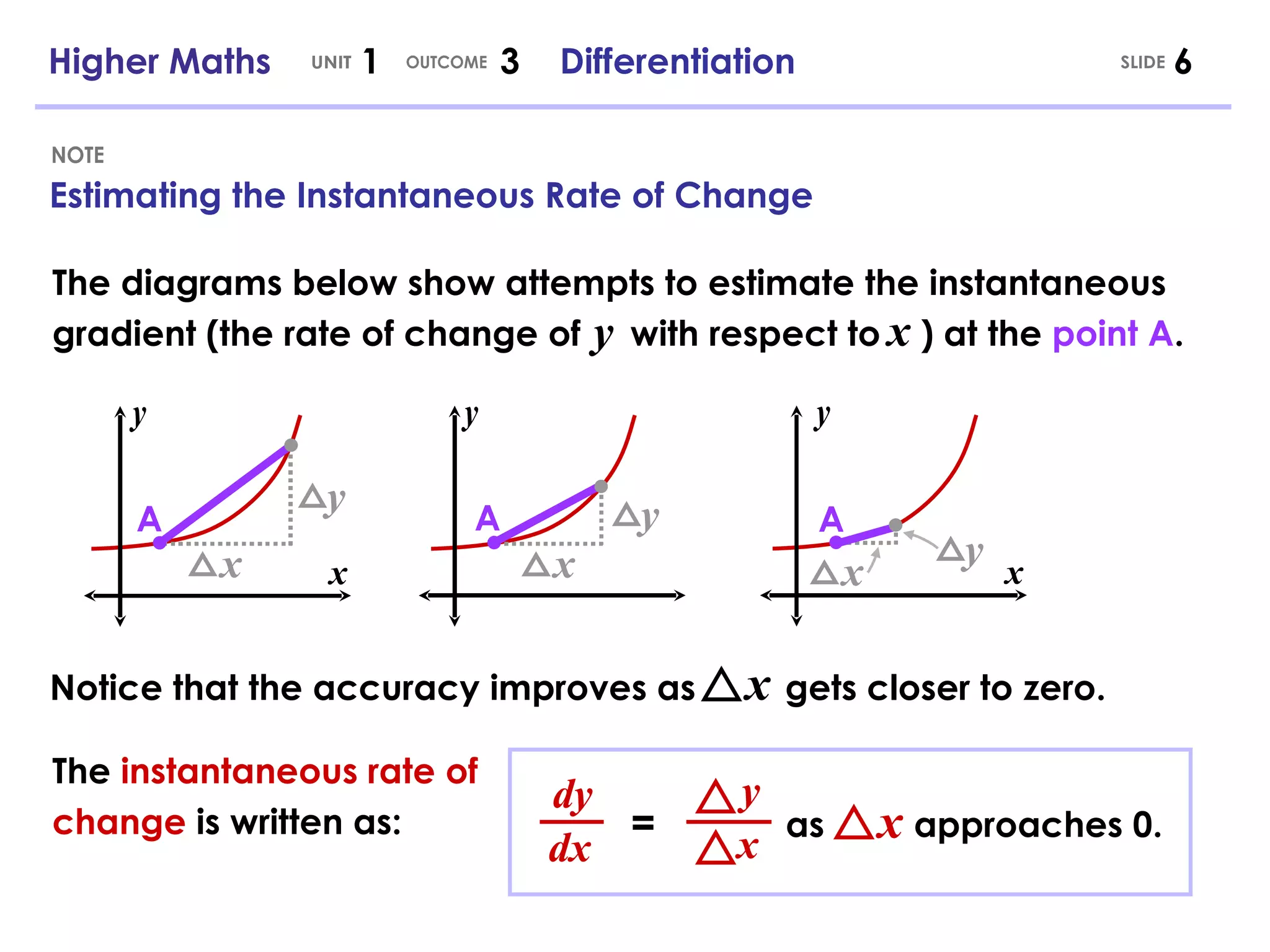
In the previous lesson, we saw a diagram where a secant line became a tangent line as the distance between the two points, , approached zero. The derivative, being the limit of the secant lines' gradients, must therefore be the gradient of the tangent line. Let's formalise this connection.
First, what exactly is a tangent line? The simple idea of a line "touching" a curve at one point can be misleading. The concept is more subtle, and calculus provides the most robust definition.
The Tangent Line and the Derivative (Calculus)
The following video from the Socratica channel, 'The Tangent Line and the Derivative,' explores the challenges of defining a tangent line and demonstrates how limits provide the solution.
Please watch from the beginning to 9:28. Pay attention to: The pitfalls of simple geometric definitions. How the tangent line is defined as the limit of secant lines (this should feel familiar!). The final, crucial connection: the derivative is explicitly defined as the gradient (slope) of the tangent line.
The video makes the connection perfectly clear:
- A secant line passes through two points on a curve. Its gradient is the average rate of change between those points, which we calculated with the difference quotient.
- A tangent line is the limit of these secant lines as the two points become one.
- The derivative at a point is the gradient (slope) of the tangent line at that point.
Let's reinforce this with a reading that uses the terminology you're familiar with.
Differentiation from first principles
This document from mathcentre.ac.uk, 'Differentiation from first principles,' formalises the link between the derivative and the gradient of a curve.
Please read Section 3, 'Differentiation from first principles of some simple curves' (page 3). Focus on the Key Point box and the explanation around Figure 3 and Figure 4. This section explicitly defines the rate of change at a point as the gradient of the tangent.
The key takeaway is that the derivative gives us a function, , which tells us the steepness of the original function, , at any given point .

Test your understanding!
In the previous lesson, we found that the derivative of is .
What is the gradient of the tangent line to the graph of at the following points?
How do these values relate to the visual shape of the parabola ?
Show answer
- At , the gradient is . The tangent line is steep and increasing.
- At , the gradient is . The tangent line is decreasing.
- At , the gradient is . The tangent line is horizontal. This corresponds to the vertex (the minimum point) of the parabola.
2. The Physical Interpretation: Instantaneous Rate of Change
The second, equally important interpretation of the derivative is as an instantaneous rate of change. This is how we move from the static picture of a graph's gradient to describing dynamic processes like motion.
Think about a car's journey. It's easy to calculate its average speed: total distance divided by total time. But what is its speed at a single instant, as shown on the speedometer? This is the "instantaneous rate of change" of distance with respect to time. When you think about it, the idea of change "in an instant" seems paradoxical. How can anything change if no time passes?
The following video from 3Blue1Brown beautifully explains this paradox and how the derivative resolves it.
The paradox of the derivative | Chapter 2, Essence of calculus
This video, 'The paradox of the derivative,' uses the example of a moving car to build an intuitive understanding of instantaneous rate of change.
Watch from the beginning to 9:44. Focus on: The paradox of 'instantaneous rate of change'. How a speedometer approximates this by measuring over a tiny, but non-zero, time interval (dt). The pure math solution: the derivative is what this approximation approaches as the time interval (dt) approaches zero.
As the video explains, the derivative isn't about what happens when (which would be meaningless). It's the limit of the average rate of change as the time interval gets infinitesimally small. This gives us the instantaneous velocity.
This concept applies to much more than just velocity. It can be the rate of change of temperature, pressure, data transfer speed in your IT work, or population growth.
Let's look at a concrete example that connects this idea of instantaneous rate of change directly back to the limit calculation and the geometry of secant and tangent lines.
2.1: Instantaneous Rates of Change- The Derivative
This text from Math LibreTexts, 'Instantaneous Rates of Change: The Derivative,' provides a great worked example of finding instantaneous velocity.
Read the text from the beginning down to 'Definition 8: Tangent Line'. Pay attention to: The amusement park ride example, which shows how calculating average velocity over smaller intervals gives a better approximation of the instantaneous velocity. The visual connection in Figure 2.2, which shows that these average velocities are the gradients of secant lines, and the instantaneous velocity is the gradient of the tangent line.
This connection is the heart of the matter. The two interpretations are two sides of the same coin:
- The instantaneous rate of change is the physical meaning.
- The gradient of the tangent line is the graphical representation of that same value.
Conclusion
In this lesson, we have given meaning to the derivative. While you learned the formal definition last time, you now understand what it truly represents.
Key Takeaways:
- Geometric Interpretation: The derivative is the gradient (slope) of the line tangent to the graph of at the given point . It tells you the steepness of the curve at that exact point.
- Physical/Analytical Interpretation: The derivative is the instantaneous rate of change of the function with respect to its variable . It describes how quickly the function's output is changing at a specific input value.
- These two ideas are unified: the gradient of the tangent line is the instantaneous rate of change.
Understanding this dual nature of the derivative is fundamental. It allows us to translate physical problems about rates of change into geometric problems about gradients, and vice versa.
In our next lesson, we will begin to move away from the cumbersome "first principles" calculations. Now that we have a solid conceptual foundation, we can start learning powerful shortcut rules for finding derivatives, beginning with the Power Rule for polynomial and power functions.