Hello! In our last lesson, we explored various metrics for evaluating model performance, like Precision and Recall. You might have noticed that these metrics often answer questions like, "Given that our model predicted 'spam', what's the probability it was actually spam?" This is a question of conditional probability.
Today, we'll dive deep into this fundamental concept and the powerful tool used to work with it: Bayes' rule. Your learning goal is to be able to explain conditional probability and Bayes' rule in the context of model predictions. Understanding this will not only clarify how metrics like Precision work but also provide the foundation for a whole class of machine learning models and a powerful framework for thinking about evidence and belief.
1. Intuition First: How Evidence Updates Beliefs
Before we get into any formulas, let's build a strong intuition. The core idea behind Bayes' rule is simple: when we get new evidence, we should update our prior beliefs; we don't start from scratch. A famous thought experiment involving "Steve the librarian" illustrates this perfectly.
The following video from 3Blue1Brown is one of the best explanations available for building this intuition.
Bayes theorem, the geometry of changing beliefs
The video "Bayes theorem, the geometry of changing beliefs" provides a brilliant, visual-first explanation of the core reasoning behind the theorem.
Please watch the following segments: The Steve example: Pay close attention to how the reasoning combines two pieces of information: the description of Steve (the evidence) and the ratio of farmers to librarians (the prior belief). From intuition to formula: This part translates the logic from the example into the formal notation of Bayes' theorem. Focus on understanding how each term in the formula maps back to the components of the "Steve" problem.
The key mantra from the video is that new evidence does not determine your beliefs in a vacuum; it should update prior beliefs. This process of updating beliefs is at the heart of Bayesian thinking.
2. The Formal Language of Bayes' Rule
Now that you have the intuition, let's formalize it. As you saw in the video, conditional probability is written as , which reads "the probability of event A happening, given that event B has already happened."
Bayes' theorem gives us a way to calculate this by "flipping" the condition:
The terms in this equation have specific names that are crucial to know:
- : Posterior Probability. This is what we want to calculate—the probability of our hypothesis being true after we've seen the evidence . It's our updated belief.
- : Prior Probability. The probability of our hypothesis being true before considering any new evidence. It's our initial belief or base rate.
- : Likelihood. The probability of observing the evidence if our hypothesis were true.
- : Evidence. The total probability of observing the evidence , regardless of whether is true or not.
This process can be visualized as a flow of information.
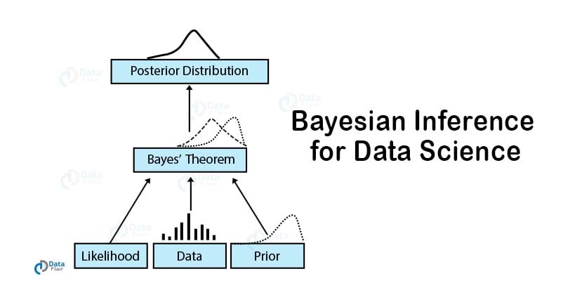
The resource below provides a great written summary of these terms and the formula.
A Gentle Introduction to Bayes Theorem for Machine ...
This article from Machine Learning Mastery clearly lays out the formula and defines the key vocabulary.
Read the first two sections: "Bayes Theorem of Conditional Probability": This provides a quick refresher on marginal, joint, and conditional probability before presenting the theorem. "Naming the Terms in the Theorem": This section defines Posterior, Prior, Likelihood, and Evidence, which is essential vocabulary.
3. Bayes' Rule in Action: The Diagnostic Test
Let's make this concrete with a classic example. This scenario is incredibly important because it reveals a common error in probabilistic reasoning known as the base rate fallacy.
Imagine a medical test for a disease.
- The disease is rare: it affects only 1 in 5000 people (0.02%).
- The test is good: it correctly identifies 85% of people who have the disease.
- The test has a false positive rate of 5%.
Question: If a random person tests positive, what is the probability they actually have the disease?
Our intuition might say 85%, but as you'll see, that's very wrong. The following sections of the article you just started will walk you through the calculation step-by-step.
A Gentle Introduction to Bayes Theorem for Machine ...
Continuing with the same article, we'll now apply the theorem to a practical problem.
Please read the sections: "Diagnostic Test Scenario": Understand the setup of the problem. "Manual Calculation": Follow the step-by-step calculation. Notice how we need to calculate P(\text{Test=Positive}) using the law of total probability. This is a common step when applying Bayes' rule. "Python Code Calculation": Review the Python code, which implements the exact logic from the manual calculation. This aligns with your preference for seeing concepts implemented in code.
The result is surprising: the probability of having the disease given a positive test is only about 0.34%! This is because the prior probability (the base rate of the disease) is so incredibly low. Even a good test with a low false positive rate will produce far more false positives than true positives when the condition it's testing for is rare.
4. Connecting Bayes' Rule to Model Predictions
So, how does this relate to the machine learning models we've been building? The connection is direct and powerful.
Let's re-frame the diagnostic test in machine learning terms:
- Hypothesis A: The patient has the disease (Actual Class = 1).
- Evidence B: The test is positive (Predicted Class = 1).
What we calculated, , is exactly the Precision of the diagnostic test!
This is a posterior probability. It's the probability of our "hypothesis" (the person has the disease) after seeing the evidence (the model predicted they do).
The article you've been reading has a fantastic section that maps all the Bayesian terms to the classifier metrics you learned in the last lesson.
A Gentle Introduction to Bayes Theorem for Machine ...
This final section from the article explicitly connects the concepts.
Read the section "Binary Classifier Terminology". Focus on the table mapping terms like True Positive Rate (TPR) and False Positive Rate (FPR) to their probabilistic counterparts like P(B|A) and P(B|\text{not } A).
This connection is not just a neat trick; it's the foundation for probabilistic classifiers. The goal of many classification models can be framed as estimating .

For example, the Naive Bayes classifier, a popular and effective algorithm, directly uses Bayes' theorem to make predictions. It's called "naive" because it makes a simplifying assumption that all the features (the data) are independent of one another. This makes calculating the likelihood computationally feasible.
Conclusion
In this lesson, you've bridged the gap between model evaluation and the underlying principles of probability. You now have a solid conceptual grasp of how to reason about model predictions in a probabilistic way.
Key Takeaways:
- Conditional Probability allows us to quantify the probability of an event given that we know another event has occurred.
- Bayes' Rule provides a formal method for updating our initial beliefs (prior) with new information (likelihood) to arrive at a refined belief (posterior). The formula is:
Posterior = (Likelihood * Prior) / Evidence. - Base Rate Fallacy is a common error where we ignore the prior probability (the base rate) and overemphasize the likelihood, leading to incorrect conclusions, as seen in the diagnostic test example.
- Connection to ML: Many familiar concepts are rooted in Bayesian probability. Precision is a posterior probability, and classifiers like Naive Bayes use the theorem directly to predict the most probable class for a given data point.
In the next module, we'll move on to a highly practical topic: Feature Engineering. While today's lesson was more theoretical, understanding the probabilistic nature of models will help you appreciate why creating informative features is so crucial for improving model performance.