Advanced Statistical Visualizations with Seaborn

1. Introducing Seaborn: Statistical Visualization Made Simple

While matplotlib gives you fine-grained control over every aspect of a plot, Seaborn automates many common statistical visualization tasks. It excels at:

• Working directly with Pandas DataFrames.
• Creating complex, multi-panel plots with simple commands.
• Providing aesthetically pleasing default styles and color palettes.

This makes it an incredibly efficient tool for the initial exploration phase of a data science project. Let's watch a short introduction to what Seaborn is and how to get started.

As you saw, Seaborn is designed for seamless integration with Pandas. We'll use its built-in datasets for the examples in this lesson. Let's start by importing our libraries and loading the "tips" dataset.

import seaborn as sns
import matplotlib.pyplot as plt
import pandas as pd




# Apply a default theme
sns.set_theme(style="whitegrid")




# Load the tips dataset
tips = sns.load_dataset("tips")
tips.head()

This will be our working dataset for the next sections.

2. Visualizing Distributions: Histograms and KDE Plots

One of the most fundamental tasks in EDA is understanding the distribution of a single variable. How are its values spread out? Are they clustered around a central point, or are there multiple peaks? The histogram is the classic tool for answering this.

A histogram groups values into a series of intervals, or "bins," and then counts how many values fall into each bin. Seaborn makes creating histograms effortless with the histplot() function.

A related visualization is the Kernel Density Estimate (KDE) plot. You can think of a KDE plot as a smoothed, continuous version of a histogram. It helps to visualize the probability density function of the variable. Seaborn can display a KDE plot on its own with kdeplot() or overlay it on a histogram for a more comprehensive view.

Let's try it ourselves. We'll create a figure and axes using the matplotlib object-oriented API you learned in the last lesson, and then tell Seaborn to draw its plot on our axes. This hybrid approach gives you the best of both worlds: Seaborn's statistical plotting power and Matplotlib's customization flexibility.

# Create a figure and axes
fig, ax = plt.subplots(figsize=(8, 6))




# Plot a histogram of the 'total_bill' column with a KDE overlay
sns.histplot(data=tips, x="total_bill", kde=True, ax=ax)




# Set the title and labels
ax.set_title('Distribution of Total Bill Amounts')
ax.set_xlabel('Total Bill ($)')
ax.set_ylabel('Frequency')

plt.show()

3. Comparing Distributions: Box Plots and Violin Plots

Histograms are great for one variable, but what if you want to compare distributions across different categories? For example, how does the distribution of total_bill differ between lunch and dinner, or across different days of the week? This is where box plots shine.

A box plot provides a concise summary of a distribution's key statistics.

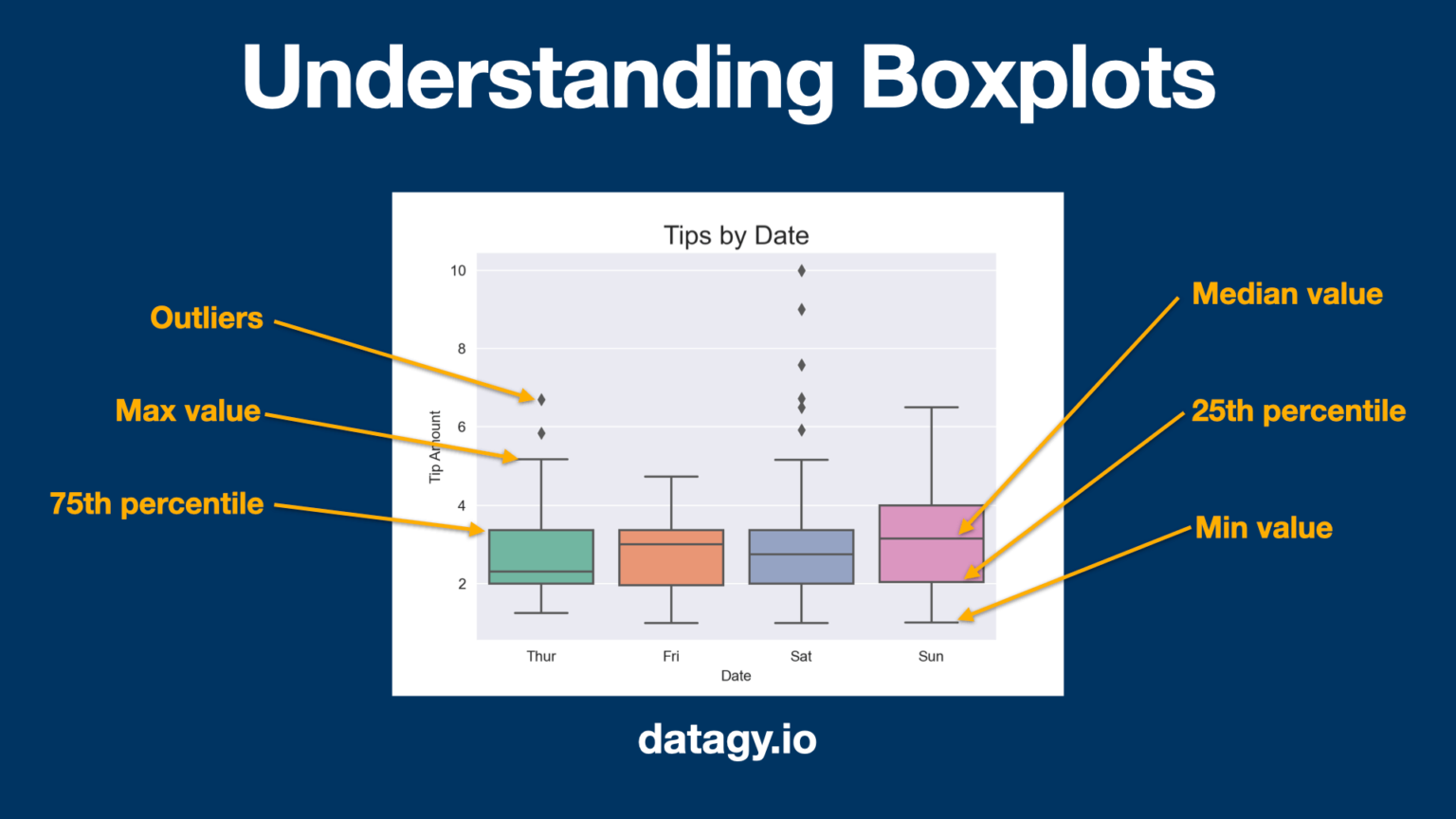
A close cousin of the box plot is the violin plot. It combines a box plot with a KDE plot, showing not only the summary statistics but also the full shape of the distribution.

Let's apply this to compare the total_bill for each day of the week. We can even add another categorical layer using the hue parameter to split the distributions by sex.

# Create a figure and axes
fig, ax = plt.subplots(figsize=(10, 7))




# Create a box plot to compare total_bill by day, split by sex
sns.boxplot(data=tips, x="day", y="total_bill", hue="sex", ax=ax)




# Set title and labels
ax.set_title('Total Bill by Day and Sex')
ax.set_xlabel('Day of the Week')
ax.set_ylabel('Total Bill ($)')

plt.show()

This single line of Seaborn code (sns.boxplot(...)) creates a visualization that would require significantly more work in matplotlib alone. You can immediately see that, on average, bills are higher on weekends and that males tend to have slightly higher bills than females across all days.

4. Visualizing Relationships: Heatmaps

Our final plot type is the heatmap. A heatmap uses color to represent the values in a 2D matrix. In data science, its most common and powerful application is to visualize a correlation matrix.

Correlation measures the linear relationship between two numerical variables, with values ranging from -1 (perfect negative correlation) to +1 (perfect positive correlation). A correlation matrix displays these values for all pairs of numerical variables in a dataset. A heatmap makes it possible to spot strong or weak relationships at a glance.

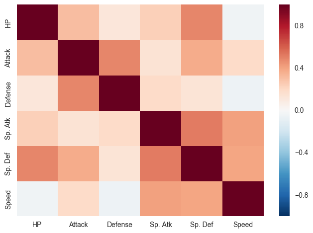
The process is straightforward:

1. Select only the numerical columns from your DataFrame.
2. Calculate the correlation matrix using the .corr() method in Pandas.
3. Plot this matrix using sns.heatmap().

Let's do this for our tips dataset.

# Create a new DataFrame with only the numeric columns from the 'tips' dataset.
# The `select_dtypes` method is a handy Pandas function for this.
numeric_tips = tips.select_dtypes(include=pd.np.number)




# Calculate the correlation matrix
correlation_matrix = numeric_tips.corr()




# Set up the matplotlib figure
fig, ax = plt.subplots(figsize=(8, 6))




# Draw the heatmap
sns.heatmap(correlation_matrix, annot=True, cmap='coolwarm', fmt=".2f", linewidths=.5, ax=ax)



# The `fmt=".2f"` argument formats the annotations to two decimal places.

ax.set_title('Correlation Matrix of the Tips Dataset')

plt.show()

From this heatmap, you can instantly see the strong positive correlation (0.68) between total_bill and tip, which confirms our intuition: larger bills tend to get larger tips.

Conclusion

In this lesson, you've added three powerful statistical plots to your data visualization toolkit. Seaborn makes it remarkably simple to generate these plots, allowing you to focus on interpreting the insights they reveal.

Key Takeaways:

• Seaborn is a high-level library that simplifies the creation of common statistical plots and works seamlessly with Pandas DataFrames.
• Histograms (sns.histplot) are essential for visualizing the distribution of a single numerical variable. Adding a KDE plot can help show a smoothed version of this distribution.
• Box plots (sns.boxplot) and Violin plots (sns.violinplot) are excellent tools for comparing distributions across different categories and identifying potential outliers.
• Heatmaps (sns.heatmap) are the standard way to visualize a correlation matrix, enabling you to quickly identify relationships between numerical variables in your dataset.

In our next lesson, we will continue exploring relationships between variables. We'll formalize the use of correlation matrices for analysis and introduce pair plots, a powerful Seaborn function that creates a grid of histograms and scatter plots to give you a comprehensive overview of your entire dataset in a single command.