Exploring Relationships: Correlation Matrices and Pair Plots

1. Correlation Heatmaps: A Deeper Look

We briefly touched on this last time, but let's formalize the concept. A correlation matrix gives us a quantitative measure of the linear relationship between pairs of numerical variables. The values in this matrix, called correlation coefficients, range from -1 to +1:

• +1: A perfect positive linear relationship. As one variable increases, the other increases proportionally.
• -1: A perfect negative linear relationship. As one variable increases, the other decreases proportionally.
• 0: No linear relationship.

A heatmap is the standard way to visualize this matrix, using color to make the patterns of correlation immediately obvious.

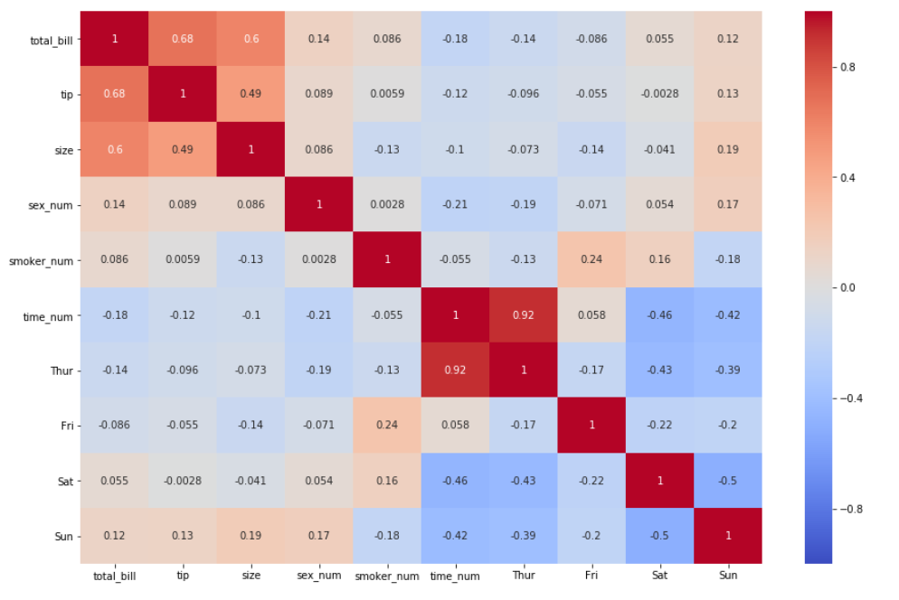
This correlation heatmap visualizes relationships in a restaurant dataset. The color bar on the right shows that warm colors (red) indicate a positive correlation, while cool colors (blue) indicate a negative one. You can quickly see a strong positive relationship between 'total_bill' and 'tip'.

While our last lesson showed how to create a basic heatmap, we can significantly improve its clarity and professionalism with a few key techniques.

Let's put this into practice using the 'penguins' dataset, which is built into Seaborn.

import pandas as pd
import numpy as np
import seaborn as sns
import matplotlib.pyplot as plt

# Load the penguins dataset and drop rows with missing values for simplicity
penguins = sns.load_dataset("penguins").dropna()

# Select only the numeric columns
numeric_penguins = penguins.select_dtypes(include=np.number)

# Calculate the correlation matrix
corr_matrix = numeric_penguins.corr()

# Set up the matplotlib figure
fig, ax = plt.subplots(figsize=(10, 8))

# --- Create the mask for the upper triangle ---
# np.triu returns the upper triangle of an array.
# np.ones_like creates an array of ones with the same shape as our matrix.
mask = np.triu(np.ones_like(corr_matrix, dtype=bool))

# --- Draw the heatmap with the mask and other improvements ---
sns.heatmap(corr_matrix, 
            mask=mask, 
            annot=True,     # Add the numbers in each cell
            vmin=-1, vmax=1, # Set the color scale limits
            cmap='coolwarm',  # Use a diverging colormap
            fmt=".2f",        # Format annotations to two decimal places
            linewidths=.5,    # Add lines between cells
            ax=ax)

ax.set_title('Triangle Correlation Heatmap of Penguin Measurements', fontsize=16, pad=12)

plt.show()

This improved heatmap is far more effective than a basic one. The diverging coolwarm palette clearly separates positive and negative correlations, and the triangular mask removes redundancy, focusing your attention on the unique relationships. You can immediately see a strong positive correlation between flipper length and body mass, and a moderate negative correlation between bill depth and bill length.

For a detailed text-based guide on these customizations, the article "How to Create a Seaborn Correlation Heatmap" (resource LINK) is an excellent reference.

2. Pair Plots: A Global View of Your Data

While a correlation heatmap gives you the numbers, it only tells you about linear relationships. What if the relationship is curved or clustered? For a more complete, qualitative overview, we use a pair plot.

A pair plot, created with sns.pairplot(), generates a grid of axes such that each numerical variable in your dataset is plotted against every other numerical variable.

• The off-diagonal plots are scatter plots, showing the relationship between two variables.
• The diagonal plots show the distribution of a single variable, typically as a histogram or a Kernel Density Estimate (KDE).

This single command gives you a comprehensive dashboard to understand your data's structure.

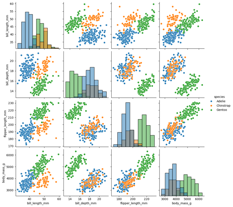
An example of a pair plot using the penguins dataset. The diagonal shows the distribution of each feature, while the scatter plots show how each pair of features relates. The points are colored by species, revealing clear clusters.

The true power of sns.pairplot() is unlocked when you add a categorical variable using the hue parameter. This colors the points in each subplot according to their category, often revealing separations or trends within groups that would otherwise be invisible.

Let's create an enhanced pair plot. For cleaner and more professional results, we'll use the corner=True argument, which, much like the mask in our heatmap, removes the redundant upper triangle.

# Create a pair plot of the penguins dataset
# We'll use 'species' to color the data points.
sns.pairplot(penguins, 
             hue='species',      # Color points by the 'species' column
             kind='scatter',       # Use scatter plots for off-diagonals
             diag_kind='kde',      # Use KDE for diagonal distributions
             corner=True,        # Only show the lower triangle and diagonal
             plot_kws={'alpha': 0.6, 's': 40, 'edgecolor': 'k'}) # Custom styles for scatter plots

plt.suptitle('Pair Plot of Penguin Measurements by Species', y=1.02, fontsize=16)
plt.show()

By running this code, you create a powerful diagnostic plot. You can instantly see that the Gentoo species (often green) is clearly separated from the other two on flipper_length_mm and body_mass_g. The relationship between bill_length_mm and bill_depth_mm also looks different for each species. These are the kinds of insights that drive feature engineering and model selection later on.

For a comprehensive written guide on all the customizations available for pair plots, including changing plot types and handling large datasets, refer to the "Seaborn Pairplot" documentation (resource LINK). It's an excellent page to bookmark for future reference.

Conclusion

In this lesson, you've learned to use two of the most important visualizations in the EDA toolkit. They provide complementary views of the relationships within your data.

Key Takeaways:

• Correlation Heatmaps provide a quantitative summary of linear relationships. Customizing them with a diverging colormap and a triangular mask makes them much more effective.
• Pair Plots provide a qualitative overview of all pairwise relationships, helping you spot both linear and non-linear patterns, as well as the distributions of individual variables.
• Using the hue parameter in a pair plot is a critical technique for understanding how relationships change across different categories in your data.
• Best practices like using corner=True or a mask create cleaner, more professional visualizations that are easier to interpret and ready for any project report or portfolio.

Now that we can visually identify strong correlations between our features, a natural question arises: what do we do about it? If two features are highly correlated, they might be providing redundant information. This issue, known as multicollinearity, can be a problem for some machine learning models. In our next lesson, we will learn how to formally diagnose it using the Variance Inflation Factor (VIF).