Summarizing Data with `groupby`

1. The Core Idea: Split-Apply-Combine

At its heart, a groupby operation is a three-step process:

1. Split: The data is split into groups based on some criteria (e.g., all rows for each unique country).
2. Apply: A function is applied to each group independently (e.g., calculate the average salary for each group).
3. Combine: The results of the function applications are combined into a new data structure (e.g., a DataFrame showing the average salary for each country).

This "Split-Apply-Combine" pattern is a cornerstone of data analysis. The image below provides a great visual summary of this flow.

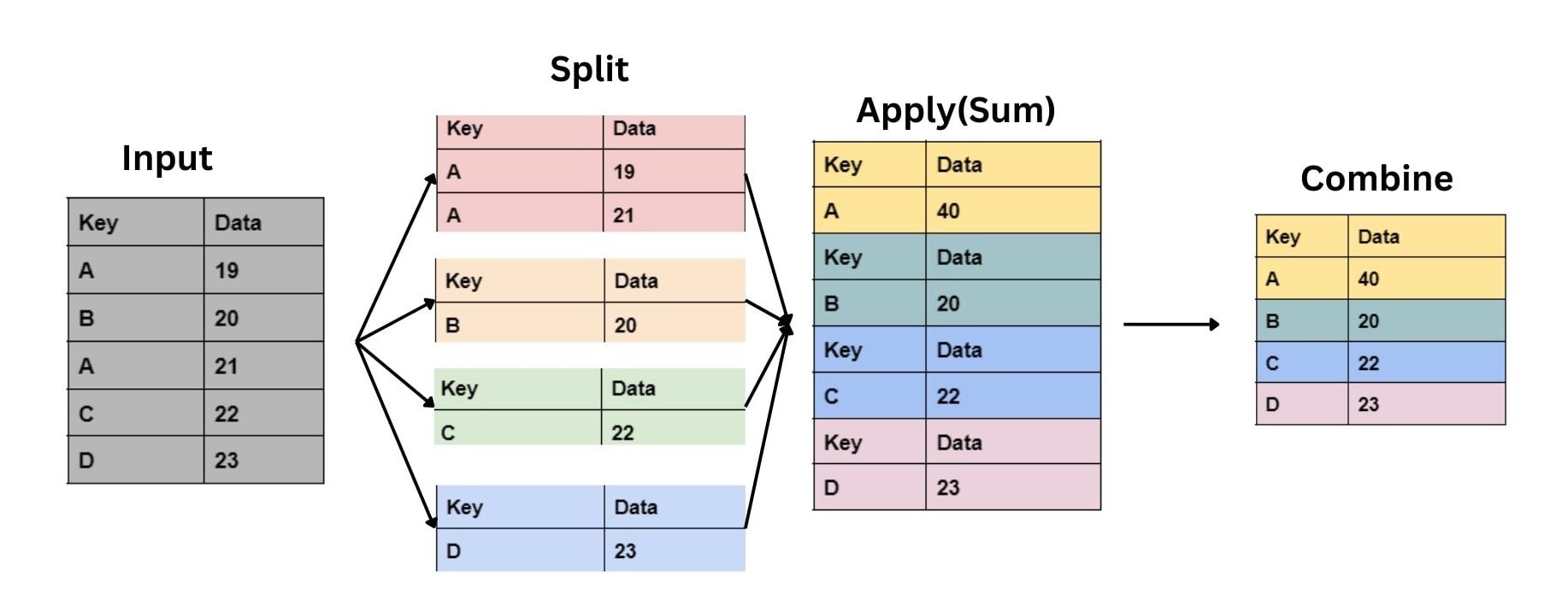
To understand how this works in Pandas, it's important to know that when you call df.groupby('some_column'), Pandas doesn't immediately compute anything. Instead, it creates a lazy DataFrameGroupBy object. This object contains all the information needed to split the data into groups. The "apply" and "combine" steps only happen when you call an aggregation method on this object.

For a deeper dive into this concept, the following reading from Real Python is excellent. It explains the mechanics and shows you how to "peek inside" a GroupBy object by iterating over it.

2. Basic Grouping and Aggregation

Let's start with the most common use case: splitting data by a single column and calculating a summary statistic. We'll use the Stack Overflow Developer Survey dataset, which you've seen before. A common question might be, "What is the typical salary for developers in different countries?"

The video below by Corey Schafer provides a clear, step-by-step demonstration of how to answer this question.

As you saw, the syntax is very intuitive: df.groupby('grouping_column')['aggregation_column'].mean().

You can use many different aggregation functions, including:

• .mean(): Average of the group
• .median(): Median of the group
• .sum(): Sum of the group values
• .count(): Number of non-null values in the group
• .size(): Total number of items in the group (including nulls)
• .nunique(): Number of unique values in the group
• .min() / .max(): Minimum and maximum values

3. Multiple Aggregations with .agg()

What if you want to calculate more than one summary statistic at a time? For instance, you might want to see both the median and mean salary for each country. Chaining .mean() and .median() won't work. For this, we use the powerful .agg() method.

The .agg() method allows you to apply multiple functions at once and gives you fine-grained control over the output.

Applying Multiple Functions

You can pass a list of function names as strings to .agg():

# Assuming 'df' is the survey data and 'country_group' is df.groupby('Country')
country_group['ConvertedComp'].agg(['median', 'mean'])

This would produce a DataFrame with both the median and mean salaries for each country.

Named Aggregations

A more modern and readable approach, especially when aggregating multiple columns, is named aggregation. This lets you specify the output column names directly, which is a huge improvement for clarity.

This image provides a perfect visual summary of the syntax for named aggregation.

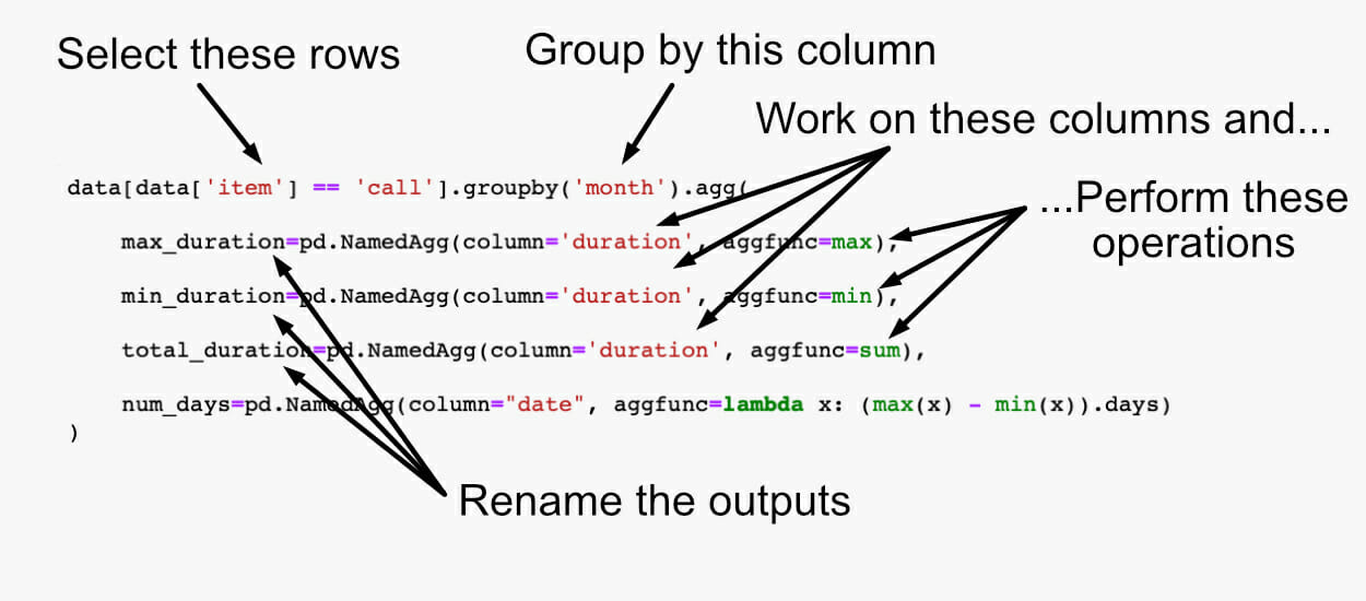
Here is a code example using the developer survey data:

import pandas as pd



# Assume 'df' is loaded with the survey data




# Group by country
country_group = df.groupby('Country')




# Use named aggregation to get median salary and number of respondents
country_summary = country_group.agg(
    median_salary=('ConvertedComp', 'median'),
    num_respondents=('Respondent', 'count')
)

print(country_summary.head())

This is the recommended way to perform complex aggregations as it makes your code self-documenting.

4. Grouping by Multiple Columns

You can also group by more than one column to create more granular subgroups. Simply pass a list of column names to groupby(). For example, to find the median salary for developers broken down by both country and their years of experience (YearsCodePro), you would do the following:

# Group by both country and years of professional coding
multi_group = df.groupby(['Country', 'YearsCodePro'])




# Calculate the median salary for each of these fine-grained groups
multi_group_summary = multi_group.agg(
    median_salary=('ConvertedComp', 'median'),
    num_respondents=('Respondent', 'count')
)




# Using .loc to view a specific combination, e.g., Germany with 5 years experience
try:
    print(multi_group_summary.loc[('Germany', '5')])
except KeyError:
    print("No data for Germany with 5 years of experience.")

The resulting DataFrame will have a MultiIndex, which is a powerful feature for working with higher-dimensional data.

5. Custom Aggregations with .apply()

Sometimes, a simple function like mean() or sum() isn't enough. What if you need to perform a more complex, custom calculation on each group? This is where the .apply() method comes in. It lets you pass any function—often a lambda function for quick, one-off operations—that will be executed on each group's DataFrame.

Let's tackle a practical problem: What percentage of developers in each country use Python?

The LanguageWorkedWith column is a string containing a list of languages. We can't just use .value_counts() on the whole column. We need to check if the string "Python" is present for each respondent within each country group. This is a perfect use case for .apply().

The following video segment walks through this exact problem, showing how to use a lambda function to perform this custom check on each group.

As the video explains, .apply() is more flexible but can be slower than the built-in, optimized aggregation functions. You should always prefer a built-in function if it can do the job, but .apply() is an indispensable tool for custom logic.

To bring everything together, let's complete the exercise from the video. The next segment shows how to combine the count of Python users with the total number of respondents to calculate the percentage. This is a great mini-project that reviews today's lesson and also uses pd.concat, which you learned last time.

Conclusion

Mastering groupby is a significant step in your journey with Pandas. It unlocks the ability to move from viewing raw data to generating powerful, aggregated insights.

Key Takeaways:

• Split-Apply-Combine: This is the mental model for all groupby operations. The groupby() method splits the data, you call a function to apply to each group, and Pandas combines the results.
• Basic Aggregations: Use simple methods like .mean(), .median(), .count(), and .sum() for quick summaries.
• .agg() for Power: Use the .agg() method for applying multiple functions at once. Prefer named aggregation for clear, readable code.
• Grouping by Multiple Columns: Pass a list of column names to groupby() to create more granular subgroups.
• .apply() for Custom Logic: When built-in functions aren't enough, use .apply() with a lambda function to run any custom code on each group.

In our next lesson, we will continue our work on data preparation by focusing on another common challenge: dealing with incorrect data types and cleaning messy string data.