Interpreting Model Predictions with SHAP and Error Analysis

1. The "Why" Behind Mistakes: Systematic Error Analysis

Imagine your best model has 92% accuracy. That's great, but what about the 8% of cases where it's wrong? Are those errors random, or is there a pattern? If you could fix the single biggest category of errors, you might gain several percentage points of performance. This is the core idea of error analysis: find the most promising areas to focus your efforts.

The following video by Andrew Ng provides a clear, practical framework for this process. It's a non-coding, conceptual guide that will shape how you approach the rest of this lesson.

This manual, systematic review is one of the most effective ways to decide what to work on next. It prevents you from spending weeks on a complex model improvement that might only fix a tiny fraction of the errors.

2. Peeking Inside the Black Box with SHAP

To understand why the model makes certain errors, we need to understand how it "thinks". SHAP (SHapley Additive exPlanations) is a state-of-the-art technique that does exactly this. It's based on a concept from cooperative game theory called Shapley values, which provide a fair way to distribute the "payout" (the model's prediction) among the "players" (the input features).

For any single prediction, SHAP tells us how much each feature value contributed to pushing the prediction from the baseline average towards its final value.

The following video provides an excellent, code-first walkthrough of the most important SHAP visualizations.

Let's break down the key plots and what they tell you.

Global Explanations: The Model's Overall Strategy

These plots summarize how the model behaves across the entire dataset.

• Bar Plot (Mean Absolute SHAP): This is your new go-to for feature importance. It shows the average impact each feature has on the model's predictions, regardless of direction.
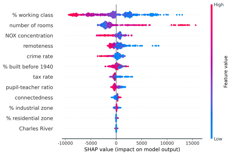
• Beeswarm Plot: This is arguably the most information-dense plot. It combines feature importance with feature effects.

Local Explanations: Debugging a Single Prediction

These plots are perfect for error analysis. They explain exactly why the model made a specific prediction for a single instance.

• Waterfall Plot: This plot shows how each feature contributes to pushing the model's output from the base value (the average prediction) to the final prediction.
• Force Plot: This is a more compact version of the waterfall plot.

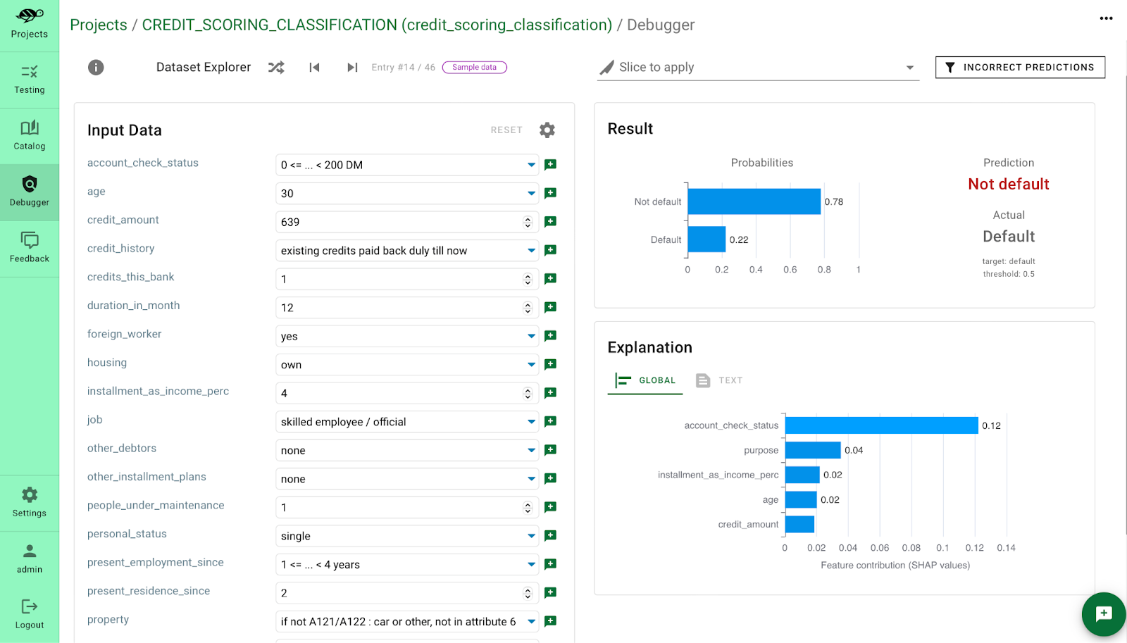
The image below shows how a local SHAP explanation could be integrated into a tool to debug an incorrect prediction. The model predicted "Not default," but the actual was "Default." The feature contribution chart immediately shows that a low account_check_status and duration_in_month were the primary drivers of this incorrect prediction.

3. Your Turn: Analyze Your Best Model

Now, let's apply this to your project. You will continue working in the same Jupyter Notebook where you selected your best model.

Instructions:

1. Install SHAP: If you haven't already, install the library: pip install shap.
2. Load Your Best Model: Load the best-performing model pipeline you identified using GridSearchCV in the last lesson. Make sure it's fitted on the full training data.
3. Compute SHAP Values:
   • SHAP explainers for tree-based models (like RandomForest or XGBoost) are optimized and work best with the underlying arrays, not the full pipeline.
   • First, process your training data (X_train) and test data (X_test) through the preprocessing part of your pipeline.

     
     
     
     # Assuming 'pipe' is your fitted pipeline
     # The preprocessor is the first step, named 'preprocessor'
     preprocessor = pipe.named_steps['preprocessor']
     X_train_processed = preprocessor.transform(X_train)
     X_test_processed = preprocessor.transform(X_test)
     
     
     
     
     # Get feature names after one-hot encoding, etc.
     feature_names = preprocessor.get_feature_names_out()
     
     
     
     
     # Get the actual model from the pipeline
     model = pipe.named_steps['model']
     

   • Create a SHAP Explainer. For tree models like XGBoost or RandomForest, use shap.TreeExplainer.

     import shap
     explainer = shap.TreeExplainer(model)
     shap_values = explainer.shap_values(X_test_processed)
     

     Note: For binary classification, shap_values will often be a list of two arrays (one for each class). For plotting, you'll typically use the values for the positive class, e.g., shap_values[1].
4. Generate and Interpret Global Plots:
   • Create a beeswarm plot to understand the overall feature impacts.

     
     
     
     # For binary classification, you might need to specify which class to explain
     shap.summary_plot(shap_values, X_test_processed, feature_names=feature_names) # For regression
     
     
     
     # shap.summary_plot(shap_values[1], X_test_processed, feature_names=feature_names) # For classification
     

   • Add a Markdown cell below the plot and write down your observations. Which features are most important? How do their values (high vs. low) affect the predictions?
5. Perform Error Analysis:
   • Get your model's predictions on the test set (X_test).
   • Create a new DataFrame containing X_test, the true labels (y_test), and the model's predictions.
   • Filter this DataFrame to get only the instances where the model was incorrect.
   • Manual Review: Look through the first 20-30 rows of this "errors" DataFrame. Try to spot patterns, just as Andrew Ng suggested. Are the errors concentrated on instances with particular characteristics?
   • Hypothesize Error Categories: Based on your review, define 3-4 potential categories of errors in a Markdown cell. For example: "errors on very low values of feature X," or "confusing class A with class B."
   • Drill Down with SHAP: Pick 2-3 specific incorrect predictions from your errors DataFrame. For each one, generate a shap.waterfall_plot or shap.force_plot to see the exact reason for the failure.

     
     
     
     # Example for the first incorrect prediction
     # Find the index of this instance in the original X_test
     error_index = errors_df.index[0] 
     original_test_index = X_test.index.get_loc(error_index)
     
     shap.waterfall_plot(explainer.expected_value[1], shap_values[1][original_test_index,:], 
                         feature_names=feature_names)
     

   • In a Markdown cell, document your findings. Did the SHAP plots confirm your hypotheses? Did they reveal something surprising about why the model failed on those instances?

Commit your updated notebook with the SHAP plots and your error analysis summary to your GitHub repository.

Conclusion

Congratulations! You've moved beyond just measuring performance and have learned how to diagnose it. This is a critical skill that separates entry-level practitioners from seasoned data scientists.

Key Takeaways:

• Model performance is more than a single metric. Understanding where a model fails is key to improving it.
• Systematic error analysis provides a structured, data-driven way to decide where to focus your development efforts.
• SHAP is a powerful tool for model explainability, providing both global insights (how the model works in general) and local insights (why a specific prediction was made).
• Combining SHAP with error analysis allows you to form hypotheses about model failures and then verify them at the individual prediction level.

In our next lesson, we will use the insights you've just generated to guide model improvements. We will also take our first step into deployment by learning how to serve our trained model through a simple REST API using FastAPI.