Welcome back to your course on becoming an internship-ready data scientist. In our last lesson, we built a solid foundation by learning how to combine data from multiple tables using JOINs and how to structure complex logic with subqueries and CTEs. We concluded by hinting at a more powerful and elegant way to solve problems like finding employees who earn more than their department's average salary.
Today, we'll explore that powerful technique: window functions. These are the workhorses of advanced SQL analytics. This lesson will teach you how to use functions like RANK, LAG, and LEAD to perform sophisticated calculations within specific subsets, or "partitions," of your data. Mastering this will enable you to solve complex business problems, from ranking products to analyzing time-series data, with surprising efficiency and clarity.
1. The Core Idea: The OVER() Clause and PARTITION BY
At its heart, a window function performs a calculation across a set of rows that are related to the current row. This "set of rows" is called a window. The OVER() clause is what defines this window, and it's what transforms a regular function (like an aggregate function) into a window function.
The most crucial part of the OVER() clause for our purposes today is PARTITION BY. This sub-clause divides the rows of your result set into smaller, independent groups, or partitions. The window function then operates on each partition separately.
A key distinction to remember is how this differs from GROUP BY:
GROUP BYcollapses multiple rows into a single summary row.- A window function with
PARTITION BYreturns a value for every single row, calculated based on the partition that row belongs to.
This video provides an excellent introduction, showing how a familiar aggregate function like MAX() can be used as a window function.
SQL Window Function | How to write SQL Query using RANK, DENSE RANK, LEAD/LAG | SQL Queries Tutorial
Watch this segment from the techTFQ channel, which clearly demonstrates the fundamental concept of window functions and partitions.
Watch from the beginning to the introduction. Pay close attention to how the OVER (PARTITION BY ...) clause allows the query to display both the individual employee details and the maximum salary for their department in the same row.
As you saw, the general syntax looks like this:
SELECT
  column_1,
  window_function() OVER (
    PARTITION BY column_to_partition_by
    ORDER BY column_to_order_by
  ) AS new_column_name
FROM your_table;
Window functions can be broadly categorized. This article provides a concise overview.
SQL PARTITION BY: Advanced Analytical Insights
This section from a Stratascratch article neatly categorizes the different types of window functions you can use with PARTITION BY.
Read the section titled "Use Cases for SQL PARTITION BY". It breaks down window functions into three main types: aggregate, ranking, and analytical. We will explore the latter two in detail next.
2. Ranking Functions: ROW_NUMBER, RANK, and DENSE_RANK
A common data analysis task is to rank items within categories—for example, ranking the top-selling products in each region or finding the top 3 employees by salary in each department. Ranking functions are designed for exactly this.
The three main ranking functions are:
ROW_NUMBER(): Assigns a unique, sequential integer to each row within a partition. No two rows will have the same number.RANK(): Assigns a rank to each row within a partition. If there are ties in the ordering value, tied rows receive the same rank, and the next rank is skipped. (e.g., 1, 2, 2, 4).DENSE_RANK(): Similar toRANK(), but if there are ties, the next rank is not skipped. (e.g., 1, 2, 2, 3).
The following video explains this crucial difference and shows a practical example.
SQL Window Function | How to write SQL Query using RANK, DENSE RANK, LEAD/LAG | SQL Queries Tutorial
Let's return to the techTFQ video to see ranking functions in action.
First, watch the ROW_NUMBER section to understand how it assigns unique numbers within each department. Then, watch from the RANK and DENSE_RANK section. Focus on the example with duplicate salaries to understand the difference between these two functions and ROW_NUMBER.
Notice that for ranking functions, the ORDER BY clause inside OVER() is mandatory. It tells the function how to determine the rank.
3. Value Functions: LAG and LEAD
Value functions, also called analytical functions, allow you to access data from other rows within your window. The two most common are LAG and LEAD.
LAG(): Accesses data from a previous row in the partition.LEAD(): Accesses data from a following row in the partition.
These are incredibly useful for calculating period-over-period changes, such as month-over-month growth in sales or the time difference between consecutive events.
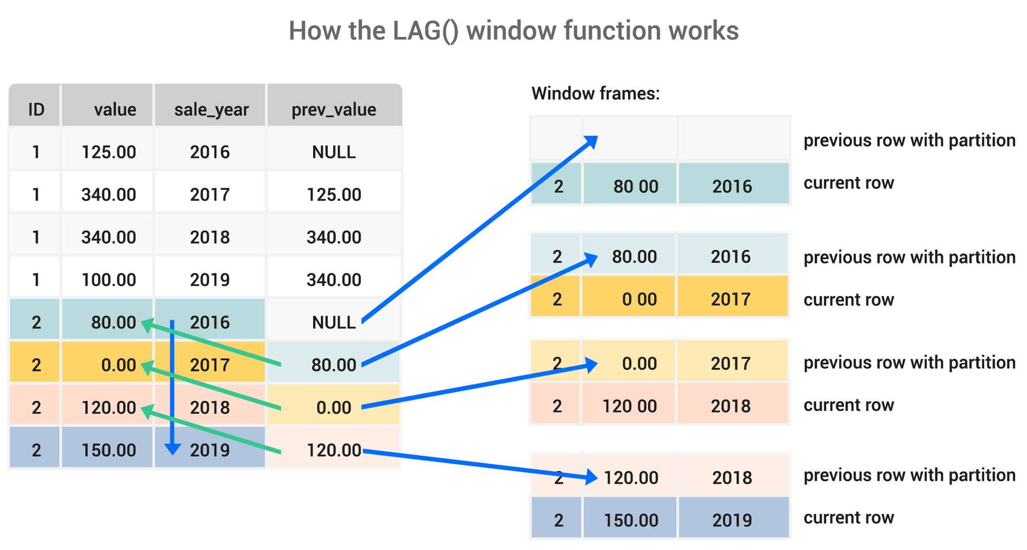
A common and powerful use case in data science is time-series analysis. The following video demonstrates how to use LAG to calculate month-over-month performance.
SQL Value Window Functions | LEAD, LAG, FIRST_VALUE, LAST_VALUE | #SQL Course 25
This video from "Data with Baraa" provides a fantastic, real-world example of using LAG for business analysis.
Watch the section on month-over-month analysis. Observe how the query is built step-by-step: first, aggregating sales by month, then using LAG to get the previous month's sales, and finally calculating the change.
Like ranking functions, LAG and LEAD require an ORDER BY clause within OVER() to establish a clear sequence of rows.
You can also provide optional arguments to LAG and LEAD:
- Offset: The number of rows to look back or forward (default is 1).
- Default Value: A value to return if the offset goes beyond the partition's boundary (default is
NULL).
The syntax is LAG(column_name, offset, default_value). For example, LAG(sales, 1, 0) would get the sales from the previous row, and if no previous row exists, it would return 0 instead of NULL.
4. Practice Exercises
Now it's your turn to apply these concepts. Below are two problems. Try to write the query to produce the "Desired Output" from the "Input" table. You can find the solutions in the collapsed sections below each problem.
The exercises use the following demand table:
| product | day | qty |
|---|---|---|
| A | 1 | 10 |
| A | 2 | 6 |
| A | 3 | 21 |
| A | 4 | 9 |
| A | 5 | 19 |
| B | 1 | 12 |
| B | 2 | 18 |
| B | 3 | 3 |
| B | 4 | 6 |
| B | 5 | 23 |
Problem 1: Find the two worst-performing days for each product
Task: Get the days corresponding to the two lowest qty values for each product.
Desired Output:
| product | day | qty | RN |
|---|---|---|---|
| A | 2 | 6 | 1 |
| A | 4 | 9 | 2 |
| B | 3 | 3 | 1 |
| B | 4 | 6 | 2 |
Solution
WITH RankedSales AS (
  SELECT
    product,
    day,
    qty,
    ROW_NUMBER() OVER (PARTITION BY product ORDER BY qty ASC) as rn
  FROM demand
)
SELECT
  product,
  day,
  qty,
  rn
FROM RankedSales
WHERE rn <= 2;
Self-correction: While RANK() or DENSE_RANK() could also work, ROW_NUMBER() is often preferred for "Top N" problems where you need exactly N results, as it handles ties by assigning distinct ranks.
Problem 2: Calculate the percentage change in quantity from the previous day
Task: For each product, calculate the percentage increase or decrease in qty compared to the previous day's qty. Order the results by day. The formula for percentage change is: .
Desired Output:
| product | day | qty | perc_increase |
|---|---|---|---|
| A | 1 | 10 | NULL |
| A | 2 | 6 | -40.00 |
| A | 3 | 21 | 250.00 |
| A | 4 | 9 | -57.14 |
| A | 5 | 19 | 111.11 |
| B | 1 | 12 | NULL |
| B | 2 | 18 | 50.00 |
| B | 3 | 3 | -83.33 |
| B | 4 | 6 | 100.00 |
| B | 5 | 23 | 283.33 |
Solution
WITH LaggedSales AS (
  SELECT
    product,
    day,
    qty,
    LAG(qty, 1, NULL) OVER (PARTITION BY product ORDER BY day) AS prev_day_qty
  FROM demand
)
SELECT
  product,
  day,
  qty,
  -- Ensure previous quantity is not zero to avoid division by zero error
  CASE
    WHEN prev_day_qty IS NOT NULL AND prev_day_qty != 0 THEN
      ROUND(((qty - prev_day_qty)::numeric / prev_day_qty) * 100, 2)
    ELSE NULL
  END AS perc_increase
FROM LaggedSales
ORDER BY product, day;
Note: The ::numeric cast is specific to PostgreSQL to ensure floating-point division.
Conclusion
In this lesson, you've unlocked one of the most powerful features in SQL for data analysis. Window functions allow you to perform complex calculations like ranking and time-series analysis without resorting to complicated self-joins or slow correlated subqueries.
Key Takeaways:
- Window functions operate on a "window" of rows related to the current row, defined by the
OVER()clause. PARTITION BYis the key to applying these functions to independent subgroups of your data, such as bydepartment,product_category, orcustomer_id.- Ranking Functions (
ROW_NUMBER,RANK,DENSE_RANK) are essential for ordering and filtering items within each partition. - Value Functions (
LAG,LEAD) are your go-to tools for comparing a row with its neighbors, forming the basis of many time-series calculations.
In our next lesson, we will delve deeper into customizing the window itself by using frame clauses. You'll learn how to compute running totals and moving averages, which are fundamental techniques in financial analysis, inventory management, and trend analysis.