Visualizing SHAP Values

1. The SHAP Summary Plot: A Bird's-Eye View of Feature Impact

While the bar plot from our last lesson gave us a simple ranking of feature importance, the summary plot provides a much richer, multi-layered view. It combines feature importance with the magnitude and direction of their effects.

This type of plot is often called a beeswarm plot because the data points are jittered to avoid overlapping, resembling a swarm of bees.

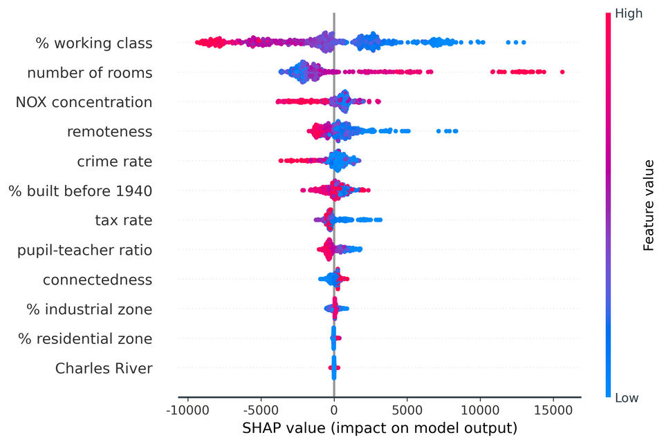
A SHAP summary (beeswarm) plot. The features are ranked by importance on the y-axis. Each dot represents a single prediction's SHAP value for that feature. The color indicates the feature's original value (high or low), and the x-axis shows the SHAP value, or the impact on the model's output.

Let's break down how to read it:

• Feature Importance: Features are ordered on the y-axis based on their global impact, with the most important feature at the top.
• Impact on Model Output: The x-axis represents the SHAP value. Points to the right of the center line have a positive SHAP value, pushing the model's prediction higher. Points to the left have a negative SHAP value, pushing the prediction lower.
• Original Feature Value: The color of each dot corresponds to the value of that feature for that data point. Typically, red indicates a high feature value, and blue indicates a low feature value.
• Correlation and Distribution: By observing the color patterns, you can infer relationships. For example, in the plot above, high values of the top feature (red dots) consistently have positive SHAP values. This tells us that higher values of that feature tend to increase the model's output.

To solidify your understanding, the following video provides an exceptionally detailed walkthrough of interpreting a summary plot. The presenter breaks it down for a few data points first, which is an excellent way to build intuition.

As you saw, the summary plot allows you to answer key questions at a glance:

• Which features are most important?
• Does a high value of a feature generally increase or decrease the prediction?
• Is the feature's effect consistent, or does it vary?

Generating this plot in Python is straightforward with the shap library. After calculating your shap_values and creating your explainer object as we did in the last lesson, you simply call summary_plot.

import shap

# Assuming 'model' is your trained model, and 'X_test' is your test data
explainer = shap.Explainer(model)
shap_values = explainer(X_test)

# Generate the summary plot
shap.summary_plot(shap_values, X_test)

Note: for classification tasks, you'll need to specify which class you are explaining, for instance shap_values[:,:,1] for the positive class.

2. The Dependence Plot: Uncovering Feature Interactions

The summary plot is excellent for an overview, but what if you want to isolate the effect of a single feature? Or, more interestingly, what if you suspect two features are interacting with each other? This is where the dependence plot shines.

A dependence plot is a scatter plot that shows the relationship between a feature's value (on the x-axis) and its corresponding SHAP value (on the y-axis).

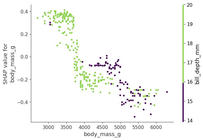
A SHAP dependence plot for the feature body_mass_g. The y-axis shows how a penguin's body mass impacts the prediction. The color of each point is determined by the value of a second feature, bill_depth_mm, revealing an interaction effect.

The true power of this plot is unlocked when we use color to represent the value of a second feature. This helps us spot interaction effects. In the plot above, notice how for a given body mass (e.g., 4000g), penguins with a high bill depth (green points) have a positive SHAP value, while those with a low bill depth (purple points) have a negative SHAP value. This indicates that the model has learned an interaction: the effect of body mass on the prediction depends on the bill depth.

Let's watch a short segment that demonstrates how to generate and interpret these plots.

To create a dependence plot, you use the shap.dependence_plot function. The interaction_index parameter is key here. If you set it to "auto", shap will automatically pick the feature that it believes has the strongest interaction with the feature you are plotting.

# Create a dependence plot for the 'RM' feature
# SHAP will automatically color it by the feature that interacts most with 'RM'
shap.dependence_plot("RM", shap_values.values, X_test, interaction_index="auto")

# You can also specify a feature to color by
shap.dependence_plot("RM", shap_values.values, X_test, interaction_index="LSTAT")

Your typical workflow for global analysis would be:

1. Start with shap.summary_plot() to get a global overview and identify the most important features.
2. For a top feature, use shap.dependence_plot() to investigate its marginal effect more closely and to automatically detect its strongest interaction.

Conclusion

In this lesson, you've added two of the most powerful explainability visualizations to your toolkit. You can now move beyond simple feature importance rankings to a more sophisticated analysis of your model's global behavior.

Key Takeaways:

• SHAP Summary (Beeswarm) Plots provide a dense overview of your model, showing feature importance, the direction of effects (positive/negative), and the distribution of impacts for every feature.
• SHAP Dependence Plots allow you to isolate the effect of a single feature and, crucially, to uncover and visualize interaction effects by coloring the plot with a second feature's values.
• Your analysis workflow should often start broad with a summary plot and then narrow down to dependence plots for features of interest.

In our next lesson, we will put this knowledge to practical use. Now that you can identify how features impact predictions, you can start to diagnose where and why your model makes mistakes. We will delve into systematic error analysis, using these insights to find specific subsets of data where your model consistently underperforms, which is the first step toward improving it.