Transaction Multiple Analysis

1. From Deal Announcement to Transaction Value

When an M&A deal is announced, the price is often stated as a "price per share." Our first task is to convert this into the total Equity Value and Enterprise Value of the transaction. This process has some important nuances that differ from our work in CCA.

Calculating Transaction Equity Value

In CCA, we used the current market capitalization. For a precedent transaction, we use the offer price.

Transaction Equity Value = Offer Price per Share × Fully Diluted Shares Outstanding

The key here is "Fully Diluted Shares Outstanding." In an acquisition, the acquirer must account for all potential shares that could be created from securities like stock options and convertible bonds.

To understand this calculation in detail, let's turn to a video that walks through the key components.

Purchase Consideration: Cash, Stock, or a Mix?

The way an acquirer pays for the target—the purchase consideration—also affects the calculation.

• All-Cash: This is the most straightforward. The offer price is a simple dollar value.
• Stock-for-Stock: The acquirer pays with its own shares. The value can be based on a fixed exchange ratio (e.g., you get 0.5 shares of AcquirerCo for every 1 share of TargetCo) or a floating exchange ratio (the ratio adjusts to deliver a fixed dollar value).
• Cash and Stock Mix: A combination of both.

Understanding these structures is essential for correctly determining the offer price.

Calculating Transaction Enterprise Value

Once you have the Transaction Equity Value, calculating the Transaction Enterprise Value (EV) is familiar.

Transaction EV = Transaction Equity Value + Net Debt (as of the deal announcement)

Remember, Net Debt = Total Debt + Preferred Stock + Non-Controlling Interest - Cash. The critical point is that we're using the transaction equity value, which already includes the control premium.

2. Standardizing the Multiples

For our multiples to be comparable, both the numerator (EV) and the denominator (e.g., EBITDA) must be standardized.

The Denominator: LTM Financials

For precedent transactions, we almost always use LTM (Last Twelve Months) financial figures as of the transaction announcement date. It is very difficult to find reliable forward-looking projections for acquired companies, and even when available, they may be inconsistent (e.g., some might include synergies, others might not).

Adjusting for Non-Recurring Items

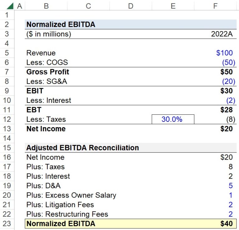
Just as with CCA, we must "normalize" the LTM financial data. This means adjusting metrics like EBITDA for any one-time or non-recurring expenses or income to reflect the company's true, ongoing profitability.

Adjusted EBITDA = Reported EBITDA + Non-Recurring Expenses - Non-Recurring Income

3. Adjusting for Premiums and Synergies

Now we arrive at the most analytical part of our task: understanding and adjusting for the specific dynamics of an M&A deal.

Calculating the Control Premium

In the last lesson, we introduced the control premium. Now, let's formalize its calculation. The premium is the percentage by which the offer price exceeds the target's unaffected share price—that is, its stock price before rumors of the deal began to influence trading.

The formula is:

$\text{Control Premium \%}=\left(\frac{\text{Offer Price per Share}}{\text{Unaffected Price per Share}}\right)-1$

Analysts typically look at the share price 1-day, 1-week, and 1-month prior to the announcement to determine a fair unaffected price.

Calculating Transaction Multiples

With the Transaction EV (numerator) and the standardized LTM financials (denominator), we can calculate the multiples. Common examples include:

• EV / LTM Revenue
• EV / LTM EBITDA
• Equity Value / LTM Net Income (P/E)

Adjusting for Synergies

As the video explained, a strategic buyer pays a price that reflects not just the target's standalone value, but also the value of the synergies it expects to create. To standardize multiples across deals with different synergy potentials, an analyst can calculate a synergy-adjusted multiple.

Synergy-Adjusted Multiple = Transaction EV / (LTM EBITDA + Expected Annual Cost Synergies)

This adjusted multiple shows the price paid relative to the future, combined earnings power of the business. It is often lower than the unadjusted multiple and gives a better sense of the "true" valuation of the standalone business plus the value attributed to synergies.

Conclusion

You have now mastered the mechanics of turning raw deal data into standardized, insightful valuation multiples. This process goes far beyond simple division; it requires a careful understanding of how transaction value is constructed and how to adjust for deal-specific factors.

Key Takeaways:

• Transaction Value: Enterprise Value in a PTA is based on the offer price, not the historical market price, and therefore incorporates the control premium.
• Standardization: To ensure comparability, you must use LTM financials as of the deal date and normalize metrics like EBITDA for non-recurring items.
• Control Premium: This is a quantifiable premium over the unaffected share price that reflects the value of control.
• Synergy Adjustments: A sophisticated analyst will adjust multiples for expected synergies to better understand the underlying valuation paid for the standalone business.

Preview of the Next Lesson:
So far in this module, we have built two distinct sets of multiples: one from living, breathing public companies (CCA) and one from historical M&A deals (PTA). In our next lesson, we will use the range of multiples from trading comps and precedent transactions to derive an implied valuation for the target company. This is where we bring everything together to create the final valuation range and the famous "football field" chart.