Implied Valuation from Multiples

Hello! Welcome to the final lesson in our module on Relative Valuation.

In the past few lessons, we've done the essential groundwork for both Comparable Company Analysis (CCA) and Precedent Transaction Analysis (PTA). You've learned how to select peer groups, find the data, and, most recently, how to calculate and standardize a set of valuation multiples. We now have two distinct sets of multiples ready for analysis.

Today, we reach the conclusion of our valuation work. Your learning outcome is to use the range of multiples from trading comps and precedent transactions to derive an implied valuation for the target company. This is the "so what?" step, where we translate all our research and calculations into a tangible range of values and, ultimately, an implied share price. We will then learn how to synthesize all our work into a single, powerful visual: the "football field" chart.

1. Applying the Multiple Ranges to Your Target

The fundamental idea of relative valuation is to apply a multiple derived from comparable companies to your target company's financial metric. Since we have a set of comparable companies for each methodology, we don't use a single multiple but rather a statistical range (e.g., the minimum, 25th percentile, median, 75th percentile, and maximum) to generate a range of implied values.

The process is as follows:

Calculate Statistics: For each multiple (e.g., EV/EBITDA), calculate the min, median, max, etc., from your peer group.
Calculate Implied Enterprise/Equity Value: Multiply this range of multiples by the target company's corresponding financial metric (e.g., LTM EBITDA) to get a range of implied Enterprise Values. For P/E multiples, you multiply by Net Income to get a range of implied Equity Values.
Bridge to Implied Share Price: For EV-based multiples, convert the Implied Enterprise Value range to an Implied Equity Value range by subtracting Net Debt. Then, divide the Implied Equity Value range by the company's fully diluted shares outstanding to get an Implied Share Price range.

Let's see this in action for both Trading Comps and Precedent Transactions.

Applying Trading Comps Multiples

Trading Comps use the multiples of currently trading public companies. The process is very dynamic and spreadsheet-driven.

Trading Comps Valuation Tutorial From Former JP Morgan Investment Banker! (Excel Template Included)

The video 'Trading Comps Valuation Tutorial' from rareliquid offers an excellent, practical demonstration of this entire process in Excel. It covers applying the multiple ranges and deriving the final share price.

Watch the segment from 34:15 to 43:55. This is the core application part of the lesson. Focus on: Calculating the Multiple Range: See how min, mean, median, and max are calculated for the peer group's multiples. Calculating Implied Value: Observe the direct multiplication of the multiple (e.g., Revenue multiple) by the target's metric (Revenue) to get the Implied Enterprise Value. Bridging to Share Price: Follow the steps of converting Implied EV to Implied Equity Value, and then dividing by the share count to arrive at the Implied Share Price.

Applying Precedent Transaction Multiples

The mechanics for Precedent Transactions are the same, but the context is different. We're using multiples from past M&A deals, which, as you know, typically include a control premium.

Precedent Transaction Analysis: The Full Guide and Excel Examples

Now, let's watch a concise explanation for Precedent Transactions from Mergers & Inquisitions. This video will reinforce the methodology you just saw, but in the context of M&A comps.

Watch from 12:24 to 14:06. Notice how the steps are identical in principle to what you saw for Trading Comps: calculate the percentile range for the multiples, multiply by the target's financials, and then bridge to the implied share price.

To solidify this calculation flow, here is a static example that lays out all the components clearly.

Precedent Transaction Analysis Model in Excel — This model from Wall Street Prep clearly shows the end-to-end process. It starts with the target's financials, uses the mean multiple from a set of comps, and applies it to calculate an Implied Transaction Value, which is then adjusted for Net Debt to arrive at the Implied Offer Value (Equity Value).

Test your understanding!

You are valuing TargetCo using Precedent Transaction Analysis.

TargetCo LTM EBITDA: $200 million
TargetCo Net Debt: $500 million
TargetCo Fully Diluted Shares Outstanding: 100 million
Your peer group of comparable transactions has a median EV / LTM EBITDA multiple of 11.0x.

Calculate the implied share price for TargetCo based on the median multiple.

Show answer

Calculate Implied Enterprise Value (Transaction Value):
- Implied EV = TargetCo LTM EBITDA × Median Multiple
- Implied EV = $200 million × 11.0x = $2,200 million
Calculate Implied Equity Value (Offer Value):
- Implied Equity Value = Implied EV - Net Debt
- Implied Equity Value = $2,200 million - $500 million = $1,700 million
Calculate Implied Share Price:
- Implied Share Price = Implied Equity Value / Shares Outstanding
- Implied Share Price = $1,700 million / 100 million = $17.00 per share

2. Summarizing the Valuation: The "Football Field" Chart

You have now produced several valuation ranges—one from Trading Comps based on EV/EBITDA, another on P/E, another from Precedent Transactions, and in a full analysis, you'd also have ranges from a DCF model. How do you present this coherently?

The industry-standard solution is the "Football Field" Chart. It's a bar chart that displays the valuation ranges from different methodologies on a single graph, allowing for easy comparison.

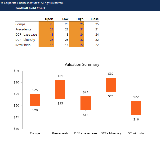
Football Field Chart for Valuation Summary — This chart is a classic example of a "Football Field." Each bar represents the valuation range (e.g., from 25th to 75th percentile) from a specific methodology. It allows you to quickly see where different valuation techniques converge or diverge, and how the current stock price compares.

Creating a professional-looking football field chart in Excel is a hallmark of a skilled financial analyst. The following resource provides a step-by-step guide.

Football Field Valuation: Excel Template, Tutorial, and Full ...

The article 'Football Field Valuation' from Breaking Into Wall Street is the definitive guide to building this chart. It explains the purpose and then walks through the Excel mechanics.

First, read the introduction to understand the chart's purpose. Then, carefully review Part 1, 'How to Make a Football Field Valuation Chart, Part 1: The Basic Chart'. The key steps are: Assemble the data: Consolidate the high and low implied share prices from each of your valuation analyses. Calculate 'distances': Prepare the data for a stacked bar chart format. Create and format the chart: Build the basic stacked bar chart and format it for clarity.

While you aren't expected to memorize these steps instantly, understanding the logic is crucial. As the article notes, in a real-world job, you will typically adapt an existing template. However, knowing how it's built from the ground up is essential for troubleshooting and customization—a skill that aligns with your goal of achieving top-tier proficiency.

3. Interpreting the Results

The football field chart is not just a presentation tool; it's an analytical one. When you look at the completed chart, you can immediately draw several conclusions:

Overall Range: It provides a defensible valuation range for the company. An analyst might conclude, "Our analysis implies a valuation between $120 and $150 per share."
Comparison of Methodologies: You can visually confirm that Precedent Transactions typically yield the highest valuation range due to the control premium.
Context for Current Price: By plotting the company's current share price as a vertical line on the chart (the "dynamic share-price line" mentioned in the advanced section of the BIWS article), you can instantly see if the company appears overvalued, undervalued, or fairly valued relative to the various methodologies.

Ultimately, valuation is as much an art as it is a science. The football field chart provides the canvas on which you apply your judgment, informed by the rigorous quantitative analysis you've performed.

Conclusion

Congratulations on completing the Relative Valuation module! You've journeyed from selecting comparable companies to calculating multiples and, today, using those multiples to derive and present a comprehensive valuation.

Key Takeaways:

An implied valuation range is derived by applying a statistical range of multiples (min, median, max) from a peer group to the target company's relevant financial metrics.
The process involves calculating an Implied Enterprise Value, bridging to an Implied Equity Value, and dividing by the share count to find the Implied Share Price range.
The "Football Field" chart is the industry standard for summarizing and comparing the valuation ranges from different methodologies (CCA, PTA, DCF, etc.) on a single page.
This summary allows you to draw a final, defensible conclusion on the company's valuation and compare it to its current market price.

Preview of the Next Lesson:
We will now pivot from the strategic, long-term perspective of valuation to the critical, short-term function of cash management. In the next module, "Cash Flow and Working Capital Management," we will begin by learning how to build a detailed 13-week direct cash flow forecast to manage short-term liquidity. This is a fundamental tool for any FP&A professional, ensuring the company has the cash it needs to operate day-to-day.