Terminal Value: Perpetuity Growth vs. Exit Multiple

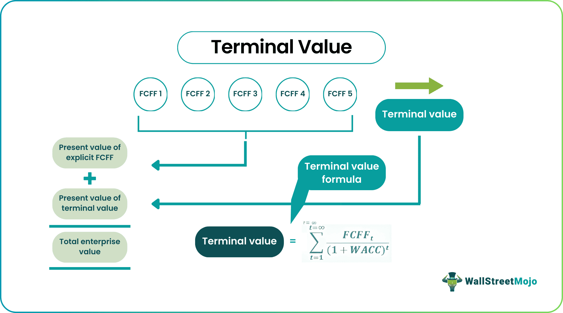
1. What is Terminal Value?

A DCF model is typically split into two stages:

1. The Explicit Forecast Period: A 5-10 year period where we build a detailed, year-by-year forecast of the company's free cash flows. The reliability of these forecasts decreases in the outer years.
2. The Terminal Period: The entire period after the explicit forecast, extending into perpetuity.

Since we cannot forecast specifics forever, we must make a simplifying assumption to calculate a single lump-sum value for all cash flows in the terminal period. This lump sum, calculated as of the end of the explicit forecast period, is the Terminal Value (TV).

We will learn the two primary methods for this calculation.

2. Method 1: Perpetuity Growth Method

This method, also known as the Gordon Growth Model, assumes that after the explicit forecast period, the company's free cash flows will grow at a constant, stable rate forever. This is analogous to a growing perpetuity, a concept you may have encountered in your MBA finance courses.

The formula is:
$\text{TV}=\frac{{\text{UFCF}}_n\times (1+g)}{\text{WACC}-g}$
Where:

• ${\text{UFCF}}_n$ is the unlevered free cash flow in the final year of the explicit forecast period (Year n).
• $g$ is the constant, perpetual growth rate.
• $\text{WACC}$ is the Weighted Average Cost of Capital, which we learned to calculate in the previous lesson.

The most critical part of this method lies in its assumptions:

• Normalized Cash Flow (${\text{UFCF}}_n$): The cash flow in the final forecast year must represent a "steady state" for the company. This means that capital expenditures should reflect a sustainable level needed for growth (i.e., capex ≈ depreciation + growth investment), and working capital should be stable. The company is assumed to have reached maturity.
• Perpetual Growth Rate ($g$): This is a highly sensitive assumption. A realistic $g$ must be a low, conservative rate. It should not exceed the long-term GDP growth rate of the country in which the company primarily operates. A common range is between 2% and 4%. If a company's growth rate were higher than the economy's forever, it would mathematically eventually become larger than the economy itself—an impossibility.

3. Method 2: Exit Multiple Method

This method takes a different approach. It assumes the company is valued or "sold" at the end of the explicit forecast period. The valuation is based on a multiple of a key financial metric, typically EBITDA, reflecting what a buyer might pay. This approach imports a relative valuation logic into our intrinsic DCF model.

The formula is:
$\text{TV}={\text{EBITDA}}_n\times \text{Exit Multiple}$
Where:

• ${\text{EBITDA}}_n$ is the Earnings Before Interest, Taxes, Depreciation, and Amortization in the final forecast year (Year n).
• $\text{Exit Multiple}$ is a valuation multiple, such as EV/EBITDA.

The key assumption here is the Exit Multiple. It is determined by analyzing:

• Comparable Public Companies: The current EV/EBITDA trading multiples of similar, mature companies in the same industry.
• Precedent Transactions: The multiples paid in recent M&A deals involving similar companies.

It's important to choose a multiple that reflects a mature company, which might be different from the multiples of high-growth companies in the peer set.

4. Application and Sanity Checks: The Art of Valuation

In practice, an analyst rarely uses one method in isolation. The best practice is to use both methods to cross-check each other and ensure the assumptions are reasonable and fall within a defensible range. This process is a critical "sanity check."

Here is the professional workflow:

1. Calculate TV with Method 1 (Perpetuity Growth): Choose a reasonable long-term growth rate $g$.
2. Calculate the Implied Exit Multiple: Take the TV from step 1 and divide it by the final year's EBITDA ($\text{TV}/{\text{EBITDA}}_n$).
3. Check: Does this implied multiple make sense when compared to the multiples of comparable companies? If it's wildly different, your growth assumption might be unrealistic.
4. Calculate TV with Method 2 (Exit Multiple): Choose a reasonable Exit Multiple based on comps.
5. Calculate the Implied Perpetual Growth Rate: Using the TV from step 4, solve for $g$ in the perpetuity growth formula. The rearranged formula is:
   $g=\frac{\text{TV}\times \text{WACC}-{\text{UFCF}}_n}{\text{TV}+{\text{UFCF}}_n}$
6. Check: Does this implied growth rate make sense? Is it below the long-term GDP growth rate? If it's too high (e.g., 6%), your exit multiple assumption is likely too aggressive.

This cross-checking procedure triangulates a reasonable Terminal Value and ensures your core assumptions are consistent with each other.

Conclusion

You have now learned how to estimate the value of a company beyond the explicit forecast period—a component that is absolutely critical to its total valuation.

Key Takeaways:

• Terminal Value (TV) captures the value of all cash flows after the explicit forecast period.
• The Perpetuity Growth Method assumes the company's cash flows grow at a constant, low rate forever. Its key driver is the perpetual growth rate ($g$).
  • $\text{TV}=\frac{{\text{UFCF}}_n\times (1+g)}{\text{WACC}-g}$
• The Exit Multiple Method assumes the company is valued at a multiple of a financial metric at the end of the forecast. Its key driver is the exit multiple.
  • $\text{TV}={\text{EBITDA}}_n\times \text{Exit Multiple}$
• Sanity checking by calculating the implied multiple from the growth method and the implied growth rate from the multiple method is the hallmark of a rigorous and defensible valuation.

With the Terminal Value estimated, we have the final piece of the puzzle. We have projected UFCFs for the explicit period and calculated the Terminal Value for the period thereafter.

In our next lesson, we will put it all together. We will learn how to discount the projected free cash flows and the terminal value to derive the enterprise value, finally arriving at a valuation for the entire company.