Hello! Welcome to the fourth lesson in our module on Financial Forecasting Techniques.
In our previous lessons, we explored forecasting a single variable based on its own history using time series methods like moving averages and exponential smoothing. This is effective for stable drivers. However, the most powerful financial forecasts are built on understanding the relationships between variables. For instance, how does marketing spend influence new customer acquisition? How does a change in interest rates affect our capital expenditure plans?
Today, we take the first step into this multivariate world. We'll learn how to statistically measure the relationships between business drivers and how to spot a common pitfall that can derail our models.
This lesson directly addresses the learning outcome: Perform correlation analysis to identify relationships between business drivers and check for multicollinearity.
1. Correlation Analysis: Measuring Relationships
Before we can build a model that says "a change in X causes a change in Y," we first need to see if X and Y even move together in a predictable way. This is what correlation analysis is for.
Correlation measures the strength and direction of a linear relationship between two variables. It's quantified by the correlation coefficient, denoted as , which ranges from -1 to +1:
- : Perfect positive correlation. When one variable goes up, the other goes up by a proportional amount.
- : Perfect negative correlation. When one variable goes up, the other goes down by a proportional amount.
- : No linear correlation. The variables don't appear to have a linear relationship.
In a business context, you might find a strong positive correlation between Advertising Spend and Website Traffic, or a negative correlation between Product Price and Units Sold.
Calculating Correlation in Excel
Excel gives us two primary ways to perform correlation analysis.
- The
CORRELFunction: For finding the correlation between two specific variables. - The Data Analysis ToolPak: For creating a correlation matrix, which efficiently shows the correlation between all pairs of variables in a dataset. This is the standard tool used in FP&A.
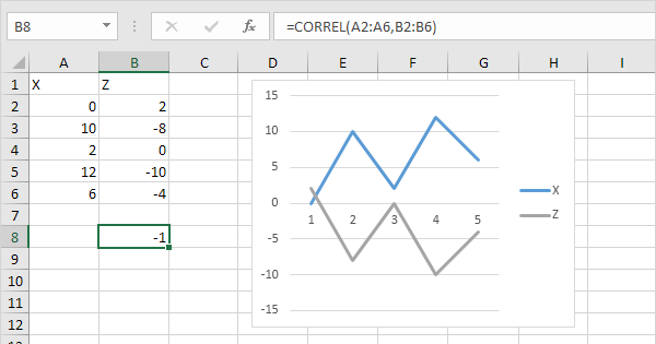
The image below shows the CORREL function in action. It calculates the correlation between variable 'X' and 'Z', resulting in -1, a perfect inverse relationship, which is also visualized in the chart.
To generate a full correlation matrix, you would:
- Ensure the Data Analysis ToolPak is enabled (
File > Options > Add-ins > Excel Add-ins > Go...). - Go to
Data > Data Analysis. - Select
Correlationand input the range containing all your numerical variables.
The output will be a table showing the correlation coefficient for every possible pair of variables. As an analyst, you would scan this matrix for high positive or negative values to identify strong relationships worth investigating further.
Test your understanding!
An FP&A analyst is examining a dataset with three potential drivers for Sales Revenue: Marketing Spend, Website Visits, and Average Discount %. The correlation matrix looks like this:
| Sales Revenue | Marketing Spend | Website Visits | Average Discount % | |
|---|---|---|---|---|
| Sales Revenue | 1.00 | |||
| Marketing Spend | 0.85 | 1.00 | ||
| Website Visits | 0.91 | 0.75 | 1.00 | |
| Average Discount % | 0.15 | 0.05 | 0.12 | 1.00 |
Based on this matrix, which two drivers seem most promising for building a predictive model for Sales Revenue?
Show answer
Website Visits (correlation of 0.91) and Marketing Spend (correlation of 0.85) are the most promising drivers. They both have very strong positive correlations with Sales Revenue, suggesting they have a significant linear relationship. Average Discount % has a very weak correlation (0.15) and is likely not a strong linear predictor on its own.
2. The Problem of Multicollinearity
Identifying drivers that are highly correlated with our target variable (like Sales Revenue) is great. But what happens when our chosen drivers are also highly correlated with each other?
This is a critical problem called multicollinearity.
For example, Marketing Spend and Website Visits are likely highly correlated with each other. If we include both in a model to predict Sales Revenue, the model will struggle to separate their individual impacts. It can't tell if an increase in sales is due to the marketing spend itself or the website visits that the spend generated.
To understand the concept and its serious consequences, let's read a short article.
Part3: Understanding Multicollinearity
This article from Prof. Frenzel, 'Part3: Understanding Multicollinearity', provides a clear, non-technical introduction to what multicollinearity is and why it's a major concern when building financial models.
Please read the sections 'What is Multicollinearity?', 'Why It’s Important to Understand Multicollinearity', and 'Causes of Multicollinearity'. Focus on how multicollinearity makes it difficult to separate the individual effects of predictors and how it inflates standard errors, making your model unreliable.
As the article explains, multicollinearity leads to two main issues for an analyst:
- Unreliable Coefficients: The model's estimates for the impact of each driver become unstable and can have wildly incorrect signs or magnitudes. You can't confidently tell a business leader, "A $1 increase in ad spend will generate $5 in revenue," because that '$5' figure could be completely wrong.
- Masked Significance: The model may fail to identify a driver as statistically significant (i.e., it will have a high p-value) even when it has a real impact. You might mistakenly discard an important business driver.
3. Detecting Multicollinearity in Excel
Now for the practical part: how do we diagnose this problem? There are two main methods.
Method 1: The Correlation Matrix (A Quick Check)
The correlation matrix you already created is your first line of defense. If you see a high correlation (as a rule of thumb, > 0.8 or < -0.8) between two of your predictor variables, you should be suspicious of multicollinearity. In our earlier example, Marketing Spend and Website Visits had a correlation of 0.75, which is getting high and warrants a closer look.
Method 2: Variance Inflation Factor (VIF) (The Standard Test)
The gold standard for detecting multicollinearity is the Variance Inflation Factor (VIF).
Conceptually, the VIF for a given predictor variable tells you how well it can be explained by all the other predictor variables. It's calculated using the formula:
Where comes from a temporary regression where you try to predict that one predictor variable using all the other predictors.
- If the other predictors can explain our variable well (high ), it means our variable is redundant. The will be close to 1, making the denominator close to 0, and the VIF will be very large.
- If the other predictors cannot explain our variable (low ), it is independent and provides unique information. The VIF will be close to 1.
The following guide provides a clear, step-by-step process for calculating VIF for each predictor variable using Excel's Data Analysis ToolPak.
The Variance Inflation Factor (VIF) is the standard metric for diagnosing multicollinearity. This guide from The Bricks, 'How to Calculate VIF in Excel', provides an excellent, practical walkthrough.
Please read the sections 'What is Variance Inflation Factor (VIF)?' and the 'Step-by-Step Guide to Calculating VIF in Excel' (Steps 1 through 6). Follow along with their example of predicting 'Monthly Sales'. The key is understanding that to get the VIF for one predictor, you must run a regression using it as the dependent variable against the other predictors.
Interpreting VIF Scores:
- VIF = 1: No correlation. The ideal situation.
- 1 < VIF < 5: Moderate correlation. Generally considered acceptable.
- VIF > 5: High correlation. A cause for concern and may require action.
- VIF > 10: Severe multicollinearity. The model's coefficients are likely unstable and untrustworthy.
4. What to Do About High VIF Scores
Detecting multicollinearity is crucial, but knowing how to address it is what makes an effective analyst. There is no single "right" answer; it requires business judgment.
Let's review the common strategies.
Now that you can diagnose the problem, let's look at the solutions. This last section of the guide outlines the most common approaches.
Please read the short section 'What To Do About High VIF Scores'. Pay attention to the different options, like removing a variable or combining them.
Here is a summary of your options when faced with a high VIF:
- Remove one of the variables. If
Marketing SpendandWebsite Visitsare highly correlated, choose one. Your choice might depend on which is easier to forecast, which has a stronger theoretical link to sales, or which is more directly controllable by the business. - Combine the variables. You could create a new, single variable. For example, you could create a "Marketing Activity Index" that is a weighted average of
Marketing SpendandWebsite Visits. This is an advanced approach but can be very powerful. - Do nothing. If your sole goal is prediction and you do not need to interpret the individual impact of each driver, multicollinearity is less of a problem. However, in FP&A, we are almost always concerned with interpretation and explaining why things are happening, so this is rarely the best option.
Conclusion
Today, you've learned a foundational skill for any data-driven analyst. You can now not only explore the relationships between different business drivers but also diagnose and address multicollinearity—a critical step in building reliable and interpretable financial models.
Key Takeaways:
- Correlation analysis uses the correlation coefficient () to measure the strength and direction of a linear relationship between two variables.
- A correlation matrix in Excel is the standard tool for quickly analyzing relationships across many variables.
- Multicollinearity is a serious issue that occurs when two or more predictor variables in a model are highly correlated with each other. It makes the model's coefficients unreliable.
- You can detect multicollinearity using a correlation matrix (as a first pass) and more definitively using the Variance Inflation Factor (VIF).
- Addressing high VIF scores often involves removing or combining correlated variables, requiring careful business judgment.
In our next lesson, we will put this all together. We will use correlation analysis to select promising drivers, check them for multicollinearity, and then build our first multiple regression model to precisely quantify their impact on a financial outcome.