Hello! Welcome to the third lesson in our module on Financial Forecasting Techniques.
In our previous lessons, we focused on driver-based forecasting. We learned to project revenue based on volume and price, and then forecast variable and fixed costs based on those same operational drivers. This is a powerful method when a clear, causal relationship exists.
But what about costs or drivers that don't have a direct link to sales volume? Think about a stable, non-production-related expense like the monthly software subscription costs for the accounting department, or the total headcount in a mature R&D division. These items might not fluctuate with every unit sold, but they aren't perfectly fixed either. Their future values are often best predicted by their own past behavior.
This brings us to today's topic: time series forecasting. We will explore techniques that use the historical data of a single variable to forecast its future.
This lesson directly addresses the learning outcome: Build time series forecasts using moving averages and exponential smoothing for stable business drivers.
1. The Intuition Behind Time Series Forecasting
Forecasting is about finding a signal in the noise. For a stable business driver, we can think of two extreme approaches:
- The Mean Model: Assume the future will be the average of all past data. This is very stable but unresponsive to any recent changes.
- The Random Walk Model: Assume the future will be whatever happened in the last period. This is highly responsive but can be misled by random, one-off fluctuations.
The truth, as is often the case, lies somewhere in between. We need a method that can smooth out random noise while still adapting to real changes in the underlying pattern.
The Simple Moving Average (SMA) is our first tool for this. It strikes a balance by averaging the m most recent data points.
To understand the core concepts and trade-offs of this approach, please start by reading an excerpt from a guide on forecasting.
Forecasting with moving averages
This document, 'Forecasting with moving averages' by Prof. Robert Nau of Duke University, provides an excellent conceptual foundation. It will help you understand the 'why' behind the technique before we jump into the 'how' in Excel.
Please read the first section, '1. SIMPLE MOVING AVERAGES' (pages 1-3). Focus on the explanation of how SMA sits between the mean and random walk models, the forecasting equation, and the critical trade-off you make when choosing the window size, 'm'.
The key takeaway is that choosing the length of your moving average (m) involves a trade-off:
- A larger
m(e.g., a 12-month moving average) creates a smoother forecast that is less affected by random noise, but it will be slower to react to real turning points. - A smaller
m(e.g., a 3-month moving average) is more responsive to recent changes but can be "jerky" and overreact to random fluctuations.
2. Moving Average Forecasting in Excel
Now let's apply this concept. Excel provides tools to calculate moving averages easily. The most common method uses the Data Analysis ToolPak, an Excel add-in you may need to enable first (File > Options > Add-ins > Excel Add-ins > Go... > Check 'Analysis ToolPak').
The following resource provides a step-by-step guide.
How to Perform Excel Data Analysis: Forecasting
This guide from ExcelDemy will walk you through the practical steps of creating a moving average forecast in Excel.
Please read 'Method 1 – Using Moving Average Method for Forecasting Data Analysis in Excel', focusing specifically on the subsection '1.1 Using Data Analysis Command'. Follow the steps to see how the ToolPak generates both the forecast values and a chart.
A moving average forecast is best suited for data that is "locally stationary"—meaning it fluctuates around a stable mean without a strong upward or downward trend.
3. A More Elegant Approach: Exponential Smoothing
The simple moving average has two intuitive drawbacks:
- It weights every observation within the window equally. Does it make sense that the data from 3 months ago is just as important as yesterday's data?
- It completely ignores all data older than
mperiods. An observation has full weight in one period and zero weight in the next, which can cause the forecast to jump.
Exponential Smoothing solves these issues. It calculates a weighted average of all past observations, with the weights decreasing exponentially as the data gets older.
The image below shows this difference visually. Notice how the Moving Average line is a "cliff"—the weight drops to zero—while the Exponential Smoothing lines show a smooth decay.
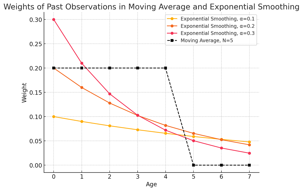
Just as m controls the SMA model, a smoothing constant, alpha (α), controls the exponential smoothing model. Alpha is a value between 0 and 1:
- A high
α(e.g., 0.8) gives a lot of weight to recent data, making the forecast very responsive. - A low
α(e.g., 0.1) gives more weight to older data, creating a much smoother forecast.
To grasp the mechanics, let's return to the conceptual guide.
Forecasting with moving averages
We will now read the section on Simple Exponential Smoothing (SES) from the same Duke University guide.
Please read '3. SIMPLE EXPONENTIAL SMOOTHING' (pages 7-10). Pay attention to the different ways the forecasting equation can be written and the concept of 'average age,' which provides a direct comparison between SMA's 'm' and SES's 'alpha'.
The core idea of Simple Exponential Smoothing (SES) can be expressed very simply:
This shows that the new forecast is a weighted average of the most recent actual data and what we had previously forecasted.
4. Exponential Smoothing in Excel
Modern Excel has a powerful, built-in function for this: FORECAST.ETS. This function automatically handles exponential smoothing and can even detect trends and seasonality.
Let's see how to use it.
How to Perform Excel Data Analysis: Forecasting
The ExcelDemy article also explains how to use Excel's modern forecasting tools, which are based on exponential smoothing.
Please read 'Method 2 – Applying FORECAST.ETS Function' and 'How to Customize Options While Forecasting'. This will show you how to use the 'Forecast Sheet' feature, which is the easiest way to generate a high-quality forecast with confidence intervals. Take note of the various options you can customize.
The Forecast Sheet tool is fantastic for quickly creating a robust forecast, complete with upper and lower confidence bounds, which is standard practice in professional FP&A presentations.
The image below illustrates how the underlying calculation works in a spreadsheet, showing the recursive nature of the formula.

5. How Do You Know if Your Forecast Is Any Good?
We have two methods (SMA and SES) and tunable parameters for each (m and α). How do we choose the best model? We need to measure the forecast error. A model is better if it produces smaller errors on average.
Common error metrics include:
- MAE (Mean Absolute Error): The average of the absolute differences between actuals and forecasts.
- RMSE (Root Mean Square Error): Similar to MAE but penalizes larger errors more heavily.
- MAPE (Mean Absolute Percentage Error): The error as a percentage of the actual value. This is extremely useful in business because it is independent of scale (an error of $100 is huge for a $500 expense, but tiny for a $1M expense).
Let's get formal definitions for these metrics.
Forecasting with moving averages
The Duke University guide provides a clear comparison table and definitions for these crucial error statistics.
Please read '2. COMPARING MEASURES OF FORECAST ERROR BETWEEN MODELS' (pages 5-6). Focus on the 'Model Comparison' table and the descriptions of RMSE, MAE, MAPE, ME, and MPE.
As an FP&A analyst, your process would be to test several models (e.g., SMA with m=3, SMA with m=6, SES with α=0.2, SES with α=0.5) and choose the one that produces the lowest error (e.g., lowest MAPE) on historical data. A critical best practice is to test this on "out-of-sample" data—data the model wasn't trained on—to ensure it predicts the future well, not just the past.
Test your understanding!
You are forecasting monthly utility expenses for an office building. The last 4 months of actual expenses were:
- Month 1: $10,000
- Month 2: $12,000
- Month 3: $11,000
- Month 4: $13,000
- Using a 3-month simple moving average (SMA), what would be your forecast for Month 5?
- Your colleague used an exponential smoothing model with
α = 0.5. Her forecast for Month 4 was $11,000. Given that the actual for Month 4 was $13,000, what is her forecast for Month 5? - Which method do you think is more appropriate if you believe last month's unexpected cold snap (causing the spike to $13,000) was a one-time event?
Show answer
-
SMA Forecast: The 3-month SMA uses the average of the last 3 actuals.
Forecast for Month 5 =($12,000 + $11,000 + $13,000) / 3 = $12,000. -
SES Forecast: Use the SES formula:
Next Forecast = α * (Last Actual) + (1-α) * (Last Forecast).
Forecast for Month 5 =0.5 * ($13,000) + (1 - 0.5) * ($11,000) = $6,500 + $5,500 = $12,000. -
If the spike was a one-time random event, a method that smooths out noise more effectively would be better. This would be a moving average with a larger
mor exponential smoothing with a lowerα. Between the two options given, both happen to yield the same result in this specific case, but conceptually, you'd want a model that is less reactive to the very last data point.
Conclusion
You have now added two powerful time series forecasting methods to your toolkit. These are indispensable for an FP&A analyst, providing a structured way to forecast stable drivers where historical patterns are the best guide.
Key Takeaways:
- Simple Moving Average (SMA) forecasts by averaging the last
mperiods. It's simple to understand but treats all points in the window equally and has a sharp data cutoff. - Exponential Smoothing (ES) forecasts using a weighted average of all past data, with weights declining exponentially. It's generally a more robust method.
- The choice of the parameter
m(for SMA) orα(for ES) determines the trade-off between smoothness and responsiveness. - In Excel, you can use the Data Analysis ToolPak for SMA and the Forecast Sheet (
FORECAST.ETS) for a more powerful exponential smoothing forecast. - Always evaluate your forecasts using error metrics like MAPE to choose the best model for your data.
In the next lesson, we will bridge the gap between driver-based forecasting and time series analysis. We will learn how to statistically test for relationships between variables using correlation analysis, which is the first step toward building sophisticated regression models to quantify the impact of key business drivers.