Hello! Welcome back to our module on Financial Forecasting Techniques.
In our last lesson, we laid a critical foundation by learning how to construct a driver-based revenue forecast using both bottom-up and top-down methodologies. You learned to deconstruct revenue into its core components of Volume × Price, giving you a powerful, operationally-grounded way to project a company's top line.
Now that we have a forecast for revenue, we must forecast the costs required to generate that revenue. This lesson builds directly on our previous work. The 'Volume' drivers we identified for our revenue forecast will now become the primary drivers for a significant portion of our costs.
Today's learning outcome is to: Forecast variable costs using unit economics and model fixed costs with step functions for capacity changes. We will dissect a company's cost structure and learn how to build a sophisticated and realistic expense forecast.
1. The Two Pillars of Cost Forecasting: Variable and Fixed Costs
As you'll recall from your MBA studies, a company's operating costs can be broadly categorized into two types:
- Variable Costs: Costs that change in direct proportion to the volume of goods or services produced.
- Fixed Costs: Costs that remain constant regardless of the volume of production, at least within a certain range.
A robust cost forecast requires separate and distinct methodologies for each. Let's begin with variable costs.
2. Forecasting Variable Costs with Unit Economics
Variable costs are directly linked to your revenue Volume driver. For every unit you sell, you incur a certain amount of cost. The core task is to determine this "cost per unit." This is where the concept of unit economics becomes central.
While our last lesson used unit economics to determine revenue per unit, we now flip the coin to look at the costs per unit. The fundamental logic is simple:
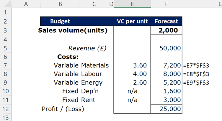
Total Variable Cost = Variable Cost per Unit × Forecasted Number of Units
The image below shows a simple Excel implementation of this logic. The variable costs for materials, labor, and energy are each calculated as a cost per unit multiplied by the total sales volume.
What Belongs in "Variable Cost per Unit"?
The challenge is to correctly identify all the costs that are truly variable. This often includes, but is not limited to:
- Cost of Goods Sold (COGS): Raw materials, direct labor.
- Transactional Fees: Credit card processing fees (e.g., 2.9% of the sale).
- Shipping & Fulfillment: The cost to pack and ship each order.
- Sales Commissions: A percentage of revenue paid to the salesperson.
To deepen our understanding, let's turn to a practical guide that breaks down the components of profitability on a per-unit basis.
Guide: understand unit economics in one day, with examples
The following article, 'Guide: understand unit economics in one day,' provides excellent examples of what constitutes a variable expense. We will focus on a specific, highly relevant section that defines these costs.
Please read the section that begins with 'Gross Profit — is the income from the user flow...'. You'll find it within 'Case one: Music Service'. Focus on the definition of variable expenses and the examples provided for different business models (mobile game, B2B software, e-commerce).
This distinction is crucial for an FP&A analyst. Mistaking a fixed cost for a variable one (or vice-versa) can lead to significant errors in forecasting profitability and cash flow, especially when modeling changes in sales volume.
A Practical Example: E-Commerce Unit Economics
Let's apply this by analyzing a case study for an e-commerce business. The process of calculating COGS per each sale is precisely the task of an FP&A analyst building a variable cost forecast.
Guide: understand unit economics in one day, with examples
Let's revisit the 'Guide: understand unit economics' article and examine the E-Bikes online store case study. It provides a clear, numerical example of calculating variable costs per unit from high-level financial data.
Please read 'Case two: E-Bikes Online Store.' Pay close attention to the steps where the author calculates 'Total COGS' and then 'COGS per each sale.' This demonstrates how you can take aggregated data from an income statement and derive the per-unit variable cost needed for your forecast.
By calculating the COGS per each sale at €3,500, the analyst has established a key driver for their variable cost forecast. They can now model the total COGS for future periods by multiplying this €3,500 by their forecast for the number of e-bikes sold (the Volume driver).
Test your understanding!
You are building a forecast for a SaaS (Software-as-a-Service) company. Based on the principles you've just read, which of the following costs would you most likely classify as variable and link to each new customer or subscription sold?
- Salaries of the core software development team.
- Hosting costs that are billed based on data usage per customer (e.g., AWS S3 storage).
- The annual rent for the company's headquarters.
- A 3% payment processing fee charged by Stripe on every subscription payment.
- A one-time sales commission paid to the account executive who closed the deal.
Show answer
The variable costs are:
- 2. Hosting costs billed based on usage: This cost scales directly with the number of customers and their activity.
- 4. Payment processing fee: This is a clear transactional cost, directly proportional to revenue.
- 5. One-time sales commission: This cost is incurred specifically for acquiring one customer.
The developer salaries and office rent are classic examples of fixed costs.
3. Forecasting Fixed Costs and the "Relevant Range"
Forecasting fixed costs is often simpler, as they don't change with production volume. Examples include administrative salaries, insurance, and rent. You might forecast them to be flat or grow at a simple inflation rate.
However, a key concept you would have encountered in your management accounting courses is the relevant range—the range of activity for which the fixed cost remains fixed. Your engineering background provides a perfect analogy: a bridge is designed to handle a certain load. Within that range, its properties are stable. But if you exceed that load, you get a catastrophic, non-linear failure.
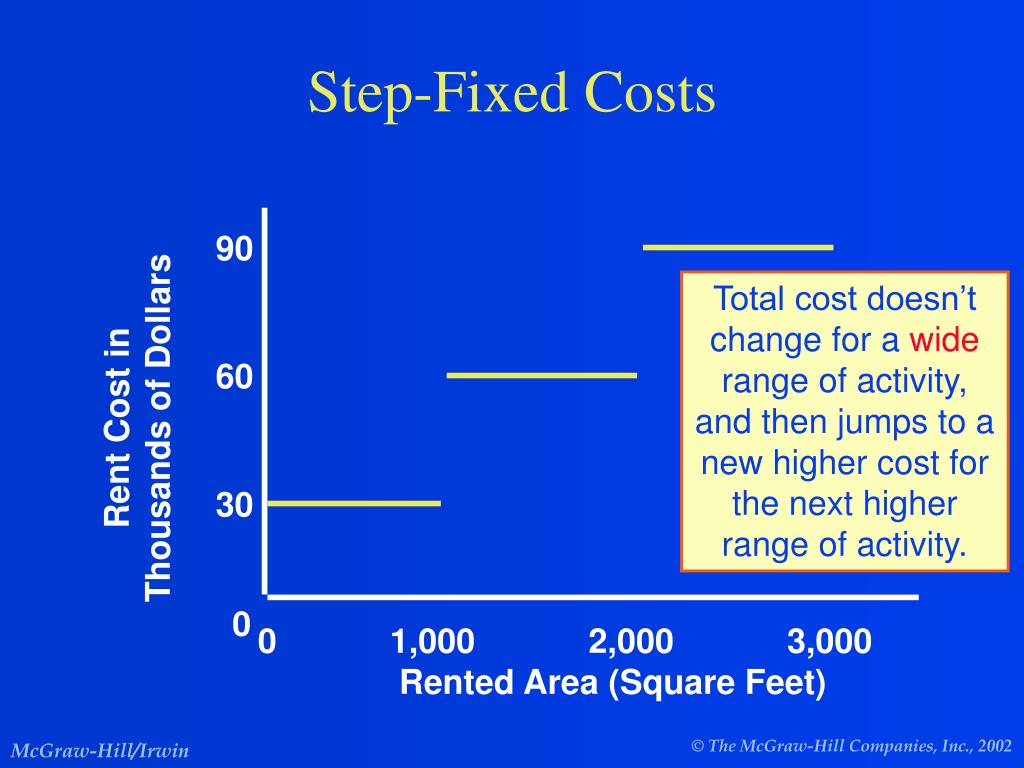
In business, exceeding the relevant range doesn't cause a collapse, but it does trigger a step-change in costs. These are called step-fixed costs.
Modeling Step-Fixed Costs
Step-fixed costs are fixed for a range of activity and then jump to a new fixed level once that range is exceeded. The graph below provides a perfect illustration.
Common business examples include:
- Production: Renting a second factory once the first one reaches 100% capacity.
- Headcount: Hiring a new accounting manager for every 20 new hires in the company.
- Support: A policy of hiring one new customer support agent for every 1,000 customers.
- IT: Adding a new server for every 10,000 active users.
As an FP&A analyst, you must model these step changes to create an accurate forecast. A simple "3% growth on all costs" assumption will fail to capture these large, lumpy increases.
Implementing Step-Fixed Costs in Excel
You can model step-fixed costs in Excel using logical functions. Let's take the customer support example: "Hire one new support agent (at a cost of $60,000/year) for every 1,000 customers."
If your forecast for the number of customers is in cell B2, a simple formula to calculate the total support cost might be:
= (B2 / 1000) * 60000
This formula is too simplistic as it assumes fractional agents. A better way is to use a function like ROUNDUP.
= ROUNDUP(B2 / 1000, 0) * 60000
This ensures you hire a whole agent as soon as the threshold is crossed.
For more complex, tiered structures (like the rent example in the image), a lookup table is a more robust and scalable solution. You would create a table with thresholds and corresponding costs, and then use VLOOKUP or XLOOKUP to find the appropriate cost for your forecasted activity level. This aligns with the best practices we discussed in our advanced Excel module.
Example Lookup Table:
| Min. Customers | Max. Customers | Support Team Cost |
|---|---|---|
| 0 | 1000 | $60,000 |
| 1001 | 2000 | $120,000 |
| 2001 | 3000 | $180,000 |
Conclusion
Today, we have added a crucial layer of depth to our forecasting ability. By dissecting costs into their variable and fixed components, you can build a model that realistically reflects the operational leverage and capacity constraints of a business.
Key Takeaways:
- Variable Costs are driven by volume. The key is to use unit economics to determine the variable cost per unit (e.g., COGS, transaction fees) and then link it to your volume forecast.
- Fixed Costs are constant within a relevant range but can increase in steps when capacity is breached.
- Step-Fixed Costs are common in business (e.g., new facilities, supervisory headcount) and must be modeled explicitly using logical or lookup functions in Excel to ensure an accurate forecast.
- A complete operating expense forecast is a blend of these different cost behaviors, all linked back to the core operational drivers of the business.
In our next lesson, we will introduce another powerful forecasting method. While we have focused on driver-based forecasting, some business drivers or costs are highly stable and predictable based on their past behavior. We will explore how to build time series forecasts using moving averages and exponential smoothing for stable business drivers.