Hello! Welcome to your next lesson in Financial Forecasting Techniques.
In our last session, we learned how to identify potential business drivers using correlation analysis and how to diagnose multicollinearity—the problem of drivers being too related to each other. This was like scouting players for a team. Today, we're going to put that team on the field and define their roles. We will build a formal model that precisely measures how each selected driver impacts our financial outcome.
This lesson focuses on the learning outcome: Execute multiple regression analysis in Excel to quantify the impact of key drivers on financial outcomes.
We'll cover how to run the analysis using Excel's built-in tools and, most importantly, how to translate the output into a concrete mathematical equation you can use for forecasting.
1. From Correlation to Regression
Correlation told us if and in which direction variables move together. Regression goes a step further: it creates an equation that quantifies that relationship.
Multiple regression analysis models the relationship between a single dependent variable (the outcome we want to predict, like Sales) and two or more independent variables (the drivers, like Advertising Spend and Number of Sales Reps).
The goal is to find the best-fitting line (or more accurately, a plane in multiple dimensions) that describes the data. The equation for this model looks like this:
Where:
- is the dependent variable (e.g., Sales Revenue).
- are the independent variables (e.g., Ad Spend, Salesforce Headcount).
- is the intercept, representing the value of when all independent variables are zero.
- are the coefficients, representing the change in for a one-unit change in the corresponding , holding all other variables constant. This is the "quantification" part we're after.
- is the error term, capturing the variability in that our model cannot explain.
Our task today is to use Excel to find the numerical values for , etc.
2. Running Multiple Regression in Excel
The primary tool for this in Excel is the Data Analysis ToolPak, which you've used before. Let's walk through the process. The following guide provides an excellent, step-by-step overview.
How to Perform Regression Analysis using Excel
This article by Jim Frost, 'How to Perform Regression Analysis using Excel', is a clear and practical guide. We will use it to learn the mechanics of running the analysis and interpreting the core output.
Please read the introduction and the sections 'Multiple Regression Analysis in Excel' and 'Step-by-Step Instructions for Filling In Excel’s Regression Box'. Pay close attention to how the data must be arranged (independent variables in adjacent columns) and how to configure the dialog box. You can also download the sample Excel file provided in the article to follow along.
To summarize and reinforce the key steps:
- Prepare Your Data: Arrange your data in columns. Your single dependent variable () can be anywhere, but all your independent variables ('s) must be in a single, contiguous block of columns. This is a specific requirement for Excel's tool.
- Launch the Tool: Go to the
Datatab and clickData Analysisin theAnalysisgroup. SelectRegressionfrom the list and click OK. - Configure the Dialog Box: This is the most important step.

- Input Y Range: Select the single column of data for your dependent variable (including the header).
- Input X Range: Select the block of columns for all your independent variables (including the headers).
- Labels: Check this box. This tells Excel that the first row of your selection contains the names of your variables.
- Output Options: Choose where you want the results to appear. Selecting
New Worksheet Plyis usually the cleanest option.
Once you click OK, Excel will generate a comprehensive summary output in a new sheet.
3. Quantifying the Impact: The Coefficients Table
The regression output contains several tables. For today, our entire focus is on the third table at the bottom, which contains the coefficients. This is where we find the values to build our equation.
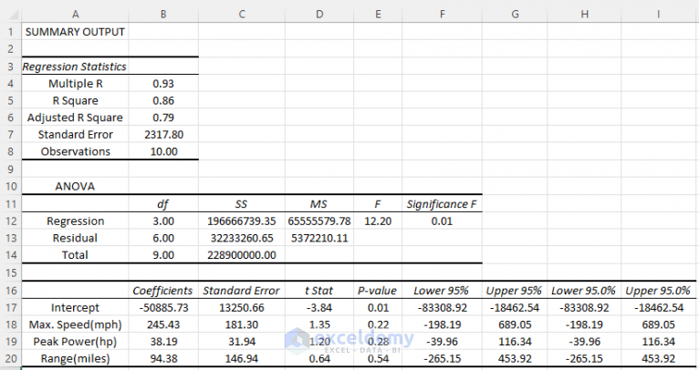
To understand how to interpret this table, let's return to our guide.
How to Perform Regression Analysis using Excel
Now let's learn how to read the results. This section of the 'Statistics by Jim' article breaks down the most important part of the output for our purpose today: the coefficients.
Please read the portion of the 'Interpreting Excel’s Regression Analysis Results' section that covers the 'Coefficients Table'. Focus on understanding the meaning of the intercept and the coefficient for each variable.
Let's distill the key information for an FP&A context:
- Intercept: This is your baseline. In the image above, the Intercept is
160.7. This means if all independent variables (Max. Speed,Peak Power,Range) were zero, the model would predict a value of 160.7 for the dependent variable. In many business scenarios, this is a theoretical starting point and may not have a practical meaning (e.g., zero advertising spend might not mean zero sales due to brand recognition). - Coefficients: These are the most powerful numbers in the output. They quantify the impact of each driver.
- The coefficient for
Peak Power(hp)is0.09. This means for every one-unit increase in horsepower, the dependent variable is predicted to increase by 0.09, assuming all other variables (Speed and Range) are held constant. - The coefficient for
Range(miles)is-0.26. This means for every one-unit increase in range, the dependent variable is predicted to decrease by 0.26, holding the other variables constant.
- The coefficient for
Building the Forecast Equation
Using the coefficients from the table, you can now write your full regression equation. For the example in the image Excel Regression Output Summary, the equation would be:
Predicted Outcome = 160.7 + (0.09 * Peak Power) - (0.26 * Range) + ... (and so on for all variables).
This equation is now a dynamic forecasting tool. If a manager asks, "What would happen to our sales if we increased our ad spend by $10,000 and hired two more salespeople?", you can plug those numbers into your equation to provide a data-driven answer.
Test your understanding!
An FP&A analyst ran a regression to predict Monthly Sales ($K) based on Ad Spend ($K) and Number of Website Clicks (in thousands). The coefficients table from the output is below:
| Coefficients | |
|---|---|
| Intercept | 50.2 |
| Ad Spend ($K) | 3.5 |
| Website Clicks (K) | 15.1 |
- Write out the full regression equation.
- Interpret the coefficient for
Ad Spend ($K). - What are the predicted
Monthly Sales ($K)if the company spends $20K on ads and gets 5,000 website clicks?
Show answer
- Equation:
Monthly Sales ($K) = 50.2 + (3.5 * Ad Spend ($K)) + (15.1 * Website Clicks (K)) - Interpretation: For every additional $1,000 spent on advertising, monthly sales are predicted to increase by $3,500, assuming the number of website clicks remains constant.
- Prediction:
Ad Spend ($K)= 20Website Clicks (K)= 5 (since the unit is in thousands)Predicted Sales = 50.2 + (3.5 * 20) + (15.1 * 5)Predicted Sales = 50.2 + 70 + 75.5Predicted Sales = 195.7- The model predicts monthly sales of $195,700.
Conclusion
Congratulations! You have just moved from simply observing relationships to quantifying them. You can now take a dataset of business drivers, execute a multiple regression analysis in Excel, and construct a predictive equation from the output. This is a fundamental building block of sophisticated driver-based financial forecasting.
Key Takeaways:
- Multiple regression models a dependent variable using multiple independent variables.
- In Excel, use the
Data Analysis ToolPakto run regression, ensuring your independent variables are in adjacent columns. - The Coefficients Table in the output provides the values for your model's intercept and the coefficient for each driver.
- Each coefficient quantifies the impact of one driver on the outcome, holding all other drivers constant.
- The final regression equation is a powerful tool for scenario analysis and forecasting.
In our next lesson, we'll address a critical question: "I have an equation, but is it any good?" We will dive into the rest of the regression output to learn how to assess our model's validity and the statistical significance of its drivers, using metrics like R-squared and p-values.