Hello! Welcome back.
In our last lesson, we built a make-or-buy model to help decide on the most cost-effective sourcing strategy. That model, like many standard financial analyses, relied on single-point estimates for variables like material costs and supplier prices. However, the real world is rarely that certain.
Today, we will address this limitation head-on. This lesson covers the learning outcome: Use Monte Carlo simulation to model the probability distribution of project outcomes and assess risk. Instead of calculating a single Net Present Value (NPV), you will learn how to generate a whole range of possible NPVs, giving you a powerful way to quantify and communicate the risk inherent in a project. This technique is a significant step up in analytical sophistication and is a hallmark of a top-tier FP&A analyst.
1. From a Single Point to a Full Picture
Traditional capital budgeting analysis, like sensitivity and scenario analysis, provides a limited view of risk. Sensitivity analysis changes one variable at a time, while scenario analysis looks at a few pre-defined outcomes (e.g., worst-case, base-case, best-case). Monte Carlo simulation overcomes these limitations by modeling thousands of possible scenarios simultaneously.

The goal is to move from a single-point answer like "The project NPV is $87,134" to a probabilistic statement like "There is a 72% probability the project will have a positive NPV, with a potential downside as low as a loss of $300,000 and an upside as high as a gain of $500,000." This provides a much richer context for decision-making.
To understand the conceptual framework and its advantages, let's begin with a short reading.
Using Monte Carlo Simulation for a Capital Budgeting Project
This article from Management Accounting Quarterly effectively contrasts Monte Carlo simulation with traditional sensitivity and scenario analyses and introduces its application in a real-world capital budgeting decision.
Read the introduction on the first page (p. 20) and the section 'Uncertainty and Risk' on page 26. Focus on: The limitations of sensitivity and scenario analysis. How Monte Carlo simulation uses probability distributions (like the triangular distribution mentioned) to model uncertainty.
2. Building a Monte Carlo Simulation in Excel
Let's translate this theory into practice. Building a Monte Carlo simulation in Excel without specialized add-ins involves four key steps:
- Build the base financial model: A standard discounted cash flow (DCF) model for a project.
- Identify uncertain variables: Determine which model inputs are not known with certainty (e.g., sales volume, variable costs, growth rates).
- Generate random inputs: Use Excel functions to replace single-point estimates with random numbers sampled from a probability distribution.
- Run simulations and collect results: Use Excel's Data Table feature to run the model thousands of times, each time with a new set of random inputs, and record the output (e.g., NPV).
The following video provides an excellent walkthrough of this entire process for a capital budgeting project. Your civil engineering background gives you a deep appreciation for how variability in inputs (like material strength or load) can affect a structure's performance; we're applying the same principle here to a project's financial performance.
Monte Carlo Simulation in Excel - Capital Budgeting
Dr. Ronald Moy's video is a clear, practical guide to implementing a Monte Carlo simulation in Excel for a capital budgeting problem. We will follow his process closely.
First, watch from 1:42 to 8:42. As you watch, I encourage you to build the simple project model in Excel yourself. Pay close attention to two key parts: The Formula for Random Cash Flows (starting at 4:46): Understand how the NORM.INV(RAND(), mean, standard_deviation) formula works. RAND() generates a random probability (from 0 to 1), and NORM.INV() finds the value on a normal distribution curve that corresponds to that probability, given a specific mean and standard deviation. Calculating a Single Simulated NPV (at 7:07): See how the standard NPV formula is applied to these newly generated random cash flows.
Now you have a model that generates a new NPV every time you press F9 (or Calculate Now). The next step is to automate this process to run thousands of trials.
Running the Simulations with a Data Table
The Data Table is a powerful, if slightly unintuitive, feature in Excel perfect for this task. It repeatedly recalculates a formula while changing an input cell. For Monte Carlo, we use a clever trick where the "input cell" is just a blank cell, which forces Excel to re-run the RAND() functions for each simulation.
Let's continue with the same video to see how this is done.
Monte Carlo Simulation in Excel - Capital Budgeting
This is the core of the hands-on exercise. You will learn how to use a Data Table to perform thousands of simulations with just a few clicks.
Watch carefully from 8:42 to 11:39. This section walks through: Setting up the column for replications (1 to 1000). Linking the output cells (NPV and IRR) at the top of the table. Highlighting the entire table range. Using the Data > What-If Analysis > Data Table tool. Remember the key step: leave the 'Row input cell' blank and select any empty cell for the 'Column input cell'.
After completing this step, you will have a column with 1,000 different possible NPVs for your project, each one representing a unique scenario for your future cash flows.
3. Analyzing the Simulation Results
You've generated the data; now comes the analysis. The goal is to distill these thousands of data points into actionable insights for management.
Descriptive Statistics and Probabilities
First, we summarize the distribution using basic statistics.
Monte Carlo Simulation in Excel - Capital Budgeting
Let's see how to summarize and interpret the simulation output.
Watch from 11:39 to the end. The video shows how to calculate the mean, median, max, and min of the simulated NPVs. This gives you a sense of the expected outcome and the range of possibilities (the best-case and worst-case scenarios from your simulation).
In your own sheet, you can calculate these statistics using the AVERAGE, MEDIAN, MAX, and MIN functions on your column of NPV results.
A crucial metric for decision-making is the probability of success. You can easily calculate this in Excel. For example, to find the probability of the project having a positive NPV, you would use the formula:=COUNTIF(results_range, ">0") / COUNT(results_range)
This tells you what percentage of your 1,000 simulated scenarios resulted in a profitable outcome.
Visualizing the Distribution
A histogram is the best way to visualize the simulation results. It groups the outcomes into bins and shows the frequency of each bin, revealing the shape of the probability distribution.
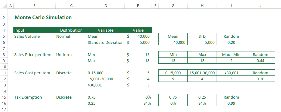
You can create a histogram in Excel using the Data Analysis ToolPak or the built-in Histogram chart type. This visual representation makes it easy to communicate the risk profile of the project to stakeholders who may not be familiar with statistical measures.
Identifying Key Risk Drivers
For a truly advanced analysis, you need to know which of your uncertain variables is causing the most volatility in the project's NPV. Is it the sales price? The growth rate? Variable costs?
Specialized software like @Risk or Crystal Ball generates a "contribution-to-variance" (or tornado) chart automatically. While building this manually in Excel is complex, understanding the concept is vital for an FP&A analyst.
Using Monte Carlo Simulation for a Capital Budgeting Project
Let's return to the Management Accounting Quarterly article, which has excellent examples of these output charts and explains their value.
Read pages 27-31, focusing on the charts and their interpretations: Figure 2 (NPV Distribution): Notice the 'Certainty' box, which shows the probability of a positive NPV (72.3%). Figure 3 (Contribution to Variance): This is the key chart. It shows that 'Number of scans in year one' accounts for 72% of the variance in NPV. This tells management exactly where the biggest risk lies. Figures 5 & 6: See how the analysis of an 'optimistic bias' changes both the probability of success and the key risk drivers. This is a powerful way to challenge assumptions.
Understanding this concept allows you to advise management on where to focus their efforts. If sales volume is the biggest risk driver, perhaps more market research is needed, or a more aggressive marketing plan could be justified to mitigate that risk.
Test your understanding!
You present a Monte Carlo simulation for a new project to your CFO. The results are:
- Mean NPV: $500,000
- Standard Deviation of NPV: $400,000
- Probability of NPV > 0: 80%
- Minimum NPV (worst-case observed): -$750,000
The CFO says, "An 80% chance of success sounds good, and the average return is great. This looks like a go." Based on the full results, what is a critical counterpoint or word of caution you should provide?
Show answer
While the average outcome is positive and the probability of success is high, the simulation reveals a significant downside risk. You should caution the CFO that there is a non-trivial chance of a substantial loss, with the worst-case scenario in the simulation showing a loss of $750,000. The high standard deviation ($400,000) relative to the mean ($500,000) also indicates a wide spread of possible outcomes. The decision to proceed depends on the company's risk appetite and whether it can absorb such a potential loss. Your role is to ensure the decision is made with a full understanding of both the potential rewards and the risks.
Conclusion
In this lesson, you have learned to move beyond deterministic financial models and embrace uncertainty. By using Monte Carlo simulation, you can provide a much more realistic and comprehensive assessment of a project's potential outcomes.
Key Takeaways:
- Monte Carlo simulation assesses risk by modeling a project's outcome thousands of times, generating a probability distribution of results (like NPV).
- In Excel, this is practically achieved using functions like
NORM.INVandRANDto model variable inputs, and theData Tablefeature to automate the simulations. - Analyzing the results involves calculating descriptive statistics (mean, min, max), determining the probability of success (e.g., P(NPV > 0)), and visualizing the distribution with a histogram.
- Advanced analysis identifies the key drivers of risk (contribution to variance), helping management focus its attention on the variables that matter most.
Preview of the Next Lesson:
Now that we can rigorously assess the risk and return profile of a single project, the next logical question is how to compare and choose between multiple competing investment opportunities. In the next lesson, you will learn how to create a summary model to compare multiple investment opportunities and support capital allocation decisions. This will involve integrating the risk analysis techniques you've learned today to make informed, strategic choices about where the company should invest its capital.