Introduction
Welcome to the next lesson in building your self-improving practice. In our previous session, you defined the key performance indicators (KPIs) that will serve as the vital signs of your consulting business, with Goal Attainment Scaling (GAS) as the cornerstone for measuring client success. You now have the what to measure. This lesson addresses the how: how to monitor these KPIs over time to distinguish meaningful changes from random fluctuations.
Our objective is to apply statistical process control (SPC) concepts to monitor your own consulting effectiveness over time. Given your background in operations research, you are already familiar with SPC as a powerful methodology for quality control in manufacturing. Here, you will repurpose that same rigorous logic to manage the quality and consistency of your own professional services. We will move beyond static reports and learn to create dynamic control charts that tell the story of your practice's performance, signaling when to intervene and when to let a stable process run.
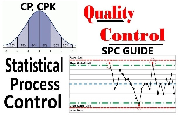
The Core Philosophy: Understanding Variation
The foundational insight of SPC, pioneered by Walter Shewhart, is that not all variation is created equal. To manage any process effectively—whether it's manufacturing a product or facilitating a client engagement—you must be able to differentiate between two types of variation.
This is arguably the most critical and often misunderstood concept in quality management. The following video provides an excellent, detailed explanation of these two types of variation and the managerial errors that arise from failing to distinguish between them.
Statistical Process Control (SPC)
This video from Quality Management & Training Limited offers a deep dive into the foundational principles of SPC.
Please watch the section explaining Shewhart's two types of causes of variation, starting from his definition of common and special causes. Pay close attention to the discussion of the two misjudgments: over-adjustment (reacting to noise) and under-adjustment (failing to react to a signal).
To summarize the key ideas from the video:
- Common Cause Variation: This is the natural, inherent, random "noise" within a stable process. For your practice, this could be the slight, unpredictable differences in GAS scores from one client to the next, even when you follow your methodology perfectly. This variation is a characteristic of the system itself. You can't eliminate it by reacting to individual data points; you can only reduce it by fundamentally improving your overall process (e.g., redesigning your intake forms, undergoing new training).
- Special Cause Variation: This is a non-random, assignable event that is not an inherent part of the process. It causes a noticeable, unpredictable shift. In your practice, this could be a new intervention technique that causes a sudden jump in client success (a positive special cause) or a period of personal burnout that leads to a clear dip in your effectiveness (a negative special cause).
The goal of SPC is to provide a statistical method to distinguish between these two, so you know when to investigate a specific cause versus when to work on improving the entire system.
Control Charts: Giving Your KPIs a Voice
The most common way to display and analyze a KPI is through a table of numbers or a simple line graph. While better than nothing, these methods make it difficult to see the difference between common and special cause variation. They tempt you to make the very over-adjustment and under-adjustment errors discussed in the video.
The control chart is the tool designed to solve this problem. It is a run chart (a graph of data over time) that includes three crucial lines:
- A Center Line (CL), which represents the process average.
- An Upper Control Limit (UCL).
- A Lower Control Limit (LCL).
Crucially, the UCL and LCL are not arbitrary goals or targets. They are calculated directly from your data and represent the natural, expected range of common cause variation. They are the "voice of the process." As long as your data points are randomly scattered between these limits, your process is considered stable and "in control." A point outside these limits signals a special cause.
The following article explains why control charts are a superior method for monitoring KPIs.
KPIs, Control Charts and Linking of Measurements - SPC for Excel
This article from SPC for Excel directly contrasts traditional KPI monitoring with the SPC approach.
First, read the section Displaying KPIs, which critiques tables and color-coded scorecards. Then, read the core section KPIs and Control Charts. This part explains how adding control limits transforms a simple run chart into a powerful diagnostic tool. Focus on the definitions of control limits and the concept of a process being in "statistical control."
Selecting the Right Control Chart for Your Practice
Now, let's connect this to the KPIs you defined in the last lesson. Different types of data require different types of control charts. Your statistics background will make this selection process straightforward. This short video provides an excellent overview and a decision tree to guide the choice.
Control Charts simply explained - Statistical process control - Xbar-R Chart, I-MR Chart,...
This video from numiqo quickly breaks down the most common control charts.
Watch from the decision tree through the explanations of the various charts. As you watch, consider where your own KPIs would fit: X-bar & R vs. I-MR charts for continuous data (like GAS scores or engagement duration). P & NP charts for discrete, pass/fail data (like the proportion of clients with a positive GAS score).
Based on the video's decision tree, here are the most logical charts for your practice:
-
For Average GAS Score per Engagement: The data is continuous. Since each completed engagement provides a single, unique average GAS score, you have a sample size of one. Therefore, the Individuals and Moving Range (I-MR) chart is the perfect tool. This will be our primary focus.
-
For Proportion of "Successful" Engagements: You might define success as any engagement with an average GAS score of 0 or greater. This is discrete, attribute data (Success/Not Success). Since the number of engagements you complete each month will vary, your sample size is variable. Therefore, a P-chart, which tracks proportions, is the appropriate choice. The research paper below validates this approach, showing how P-charts are used in healthcare to monitor professional performance.
Application of Statistical Process Control Methods to Monitor ... - PMC
This paper from the American Medical Informatics Association Proceedings demonstrates the application of SPC in a professional service context.
Read the section on Methods, which specifically describes using a P-chart for analyzing proportions of guideline-concordant decisions. Then, review the Conclusion, which affirms that control charts are more sensitive for detecting changes than simple before-after comparisons.
A Practical Walkthrough: Creating an I-MR Chart for GAS Scores
Let's build an I-MR chart for your main KPI: the average Goal Attainment Score per client engagement. Imagine you have the following scores from your last 20 completed engagements, pulled from your Airtable database:
| Engagement # | Avg GAS |
|---|---|
| 1 | 0.8 |
| 2 | 1.1 |
| 3 | 0.5 |
| 4 | -0.2 |
| 5 | 1.5 |
| 6 | 0.9 |
| 7 | 1.2 |
| 8 | 1.0 |
| 9 | 0.7 |
| 10 | 1.8 |
| 11 | 0.6 |
| 12 | 0.4 |
| 13 | 0.1 |
| 14 | -0.5 |
| 15 | -0.7 |
| 16 | 0.0 |
| 17 | -0.4 |
| 18 | 0.2 |
| 19 | 0.3 |
| 20 | 0.5 |
Here is the step-by-step process to turn this data into a control chart.
1. Calculate the Center Line (CL):
The center line for the Individuals (I) chart is simply the average of all your data points.
So, your CL = 0.59.
2. Calculate the Moving Ranges (MR):
The moving range is the absolute difference between consecutive data points. You'll have n-1 moving ranges.
- ...and so on.
3. Calculate the Average Moving Range:
4. Calculate the Control Limits (UCL and LCL):
The control limits for an Individuals chart are calculated using the average moving range. The formulas are:
The constant 2.66 is derived from , where is a control chart constant (1.128 for a moving range of size 2). This is the standard "3-sigma" limit for I-MR charts.
Using our data:
5. Plot and Interpret the Chart:
You would now plot your 20 GAS scores, the CL at 0.59, the UCL at 2.34, and the LCL at -1.16.
In this hypothetical data, all points fall between the UCL and LCL. This indicates your process is in statistical control. The variation you see is common cause variation. Your practice, on average, produces a GAS score of 0.59, with a predictable range between -1.16 and 2.34.
Now, imagine engagement #10 was 2.5 instead of 1.8. This point would be above the UCL of 2.34. This would be a special cause. Your action would be to investigate: what went exceptionally well with client #10? Did they have a unique motivation? Did you try a new technique that was highly effective? Can you replicate it? This is data-driven learning. Conversely, a point below the LCL would trigger an investigation into what went wrong.

Conclusion
In this lesson, you've bridged the gap from static KPIs to dynamic process monitoring. By applying the principles of Statistical Process Control, you can now analyze the performance of your consulting practice with the same rigor you might apply to a simulation or experiment.
Key Takeaways:
- SPC distinguishes between common cause variation (the natural noise in your stable process) and special cause variation (a signal that something has fundamentally changed).
- Control charts are the essential tool for this, using statistically derived limits (UCL/LCL) to visualize process stability. They are superior to simple tables or dashboards.
- For a KPI like the average GAS score per client, the I-MR chart is the ideal tool. For tracking the proportion of successful clients, the P-chart is appropriate.
- Interpreting a control chart allows you to make informed decisions: investigate special causes to learn from successes and failures, and implement systemic changes to reduce common cause variation and improve overall performance.
You now have a powerful tool for ongoing self-assessment. In our final lesson for this module, you will learn how to integrate this continuous monitoring into a periodic, structured review. We will focus on how to conduct a quarterly practice review using a structured, data-informed self-assessment template, where your new control charts will be a star exhibit.