Summarizing Candidate Data with PivotTables

1. Creating Your First PivotTable

Before you can analyze your data, you need to summarize it. A PivotTable is the perfect tool for this. The first step is to insert one based on your MasterTracker table.

Because you have already structured your data as an Excel Table, you're perfectly set up. Excel will automatically recognize the entire data range and know that any new data you add later should be included when the PivotTable is refreshed.

To get a foundational understanding of how PivotTables work, let's start with a comprehensive video guide.

Your Turn: Insert a PivotTable

1. Open the MasterTracker Excel file that you enhanced in the last lesson.
2. Click any single cell inside your MasterTracker table.
3. Go to the Insert tab on the ribbon and click PivotTable.
4. A dialog box will appear. The Table/Range should already show your table name (e.g., MasterTracker).
5. Ensure New Worksheet is selected. This keeps your summary report separate from your raw data, which is a best practice.
6. Click OK.

You will now see a new worksheet with a PivotTable placeholder on the left and the PivotTable Fields pane on the right. This pane is your control panel for designing the report.

2. Building the Summary: Counts by Stage and Recruiter

Our goal is to create a report that shows two things simultaneously: how many candidates are in each stage, and which recruiter is managing them. This requires a two-dimensional summary.

First, let's get a simple count of candidates for each Current Stage.

Activity: Count Candidates by Stage

1. In the PivotTable Fields pane, find the Current Stage field. Drag it into the Rows area at the bottom of the pane. You'll see the stages (Screening, Interview, Offer, etc.) appear as row labels in your PivotTable.
2. Next, we need to count the candidates. A common and reliable method is to use a unique identifier. Drag the Candidate ID field into the Values area.
3. Crucially, Excel might default to Sum of Candidate ID. This doesn't make sense; we need to count the candidates, not sum their IDs.
   • Click on Sum of Candidate ID in the Values area.
   • Select Value Field Settings.
   • In the dialog box, change the calculation from Sum to Count.
   • Click OK.

Your PivotTable now shows a count of candidates in each recruitment stage.

Activity: Add the Recruiter Dimension

Now, let's add the Recruiter breakdown.

1. Find the Recruiter field in your field list.
2. Drag the Recruiter field into the Columns area.

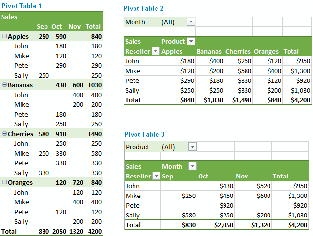
Instantly, your PivotTable transforms into a matrix. You now have Current Stage running down the rows, Recruiter names across the columns, and the count of candidates at the intersection of each. This is a classic MIS report format that provides a huge amount of information at a glance.

3. Alternative Method: Using Your Counter Columns

In the last lesson, you created helper columns like Hired Counter, Rejected Counter, and Active Counter. This was strategic preparation for this exact moment. Using these columns can make summarizing even faster.

Let's see how. We will create a simple summary of Hired, Rejected, and Active candidates by recruiter.

Activity: Summarize with Counter Columns

1. Clear your existing PivotTable by dragging all the fields out of the four areas (Rows, Columns, Values, Filter).
2. Drag Recruiter to the Rows area.
3. Now, drag Active Counter, Hired Counter, and Rejected Counter one by one into the Values area.

Notice that Excel defaults to Sum for each of these. In this case, that's exactly what we want! Since the columns contain a 1 for the correct status and 0 otherwise, summing them up gives a perfect count. This method is explicit and removes the step of changing the value field setting.

This technique is especially useful when you want to show specific, pre-defined categories as columns in your final report, as we've done here.

4. Finalizing Your Report

A raw PivotTable is functional, but for an MIS report, presentation matters. Let's apply a few professional touches.

Your Turn: Polish the PivotTable

Let's return to your main PivotTable (with Current Stage in Rows and Recruiter in Columns).

1. Clean up Empty Cells: You may see (blank) values. It’s cleaner to show these as 0.
   • Right-click anywhere in the PivotTable.
   • Choose PivotTable Options.
   • On the Layout & Format tab, check the box for For empty cells show: and type 0. Click OK.
2. Rename Headers: The default headers like "Row Labels" and "Column Labels" are unprofessional.
   • Simply click on the cell that says "Row Labels" and type a better title, like Pipeline Stage.
   • Do the same for "Column Labels" and rename it to Recruiter.
3. Apply a Style:
   • Click anywhere in your PivotTable.
   • Go to the Design tab that appears.
   • Explore the PivotTable Styles gallery and pick a clean, professional-looking style. This simple step greatly improves readability.
4. Refresh Data: This is a crucial final point. If you go back to your MasterTracker and add or change any data, the PivotTable will not update automatically. You must manually refresh it.
   • Right-click the PivotTable and select Refresh. (Alternatively, go to the Data tab and click Refresh All).

Conclusion

Excellent work! You have successfully transformed a detailed data tracker into a powerful, interactive summary report. This is a fundamental skill for any MIS role, allowing you to quickly answer key business questions directly from source data.

Here are your key takeaways from this lesson:

• A PivotTable is the fastest way to summarize large datasets in Excel.
• You build reports by dragging fields into the Rows, Columns, and Values areas.
• When counting items like candidates, you must change the Value Field Settings from the default Sum to Count.
• You can create powerful two-dimensional summaries by using both the Rows and Columns areas.
• Using pre-calculated helper columns (like your Hired Counter) can simplify and speed up PivotTable creation.
• Always format and refresh your PivotTable to ensure it is clean, professional, and up-to-date.

Your MasterTracker is now feeding a powerful summary report. In our next lesson, we will bring this data to life by creating visualizations. You will learn how to create a dashboard to visualize recruitment funnel metrics and recruiter performance, turning your summary table into an insightful and interactive tool for management.