Introduction
Welcome back to the recruitment pipeline capstone project. In our last lesson, you successfully built a MasterTracker by using Power Query to automatically consolidate data from multiple recruiter files. This is a huge time-saver and a critical skill for an MIS Executive.
Today, we'll build on that foundation. Our learning outcome is to enhance the tracker with calculated columns for time-in-stage and current status (Active, Hired, Rejected). Raw data, like an application date, is useful, but it doesn't tell the full story. By adding calculated columns, we can transform this raw data into powerful metrics that answer key business questions:
- How long has a candidate been in our pipeline?
- What is the candidate's current status in simple terms?
- How long did it take us to make a hiring decision?
These metrics are the building blocks for the summary reports and dashboards you'll create later. Let's start transforming your data tracker into an analytical tool.
1. Calculating "Days in Pipeline"
The first and most fundamental metric is tracking how long each candidate has been in the recruitment process. This helps recruiters prioritize follow-ups and gives managers visibility into pipeline velocity. We'll add a column to calculate the number of days from the Application Date to today.
There are two common ways to do this in Excel.
Method 1: Simple Subtraction with TODAY()
You can subtract the Application Date from today's date. The TODAY() function in Excel always returns the current date.
=TODAY()-[@[Application Date]]
This formula works perfectly, but you might need to format the result as a 'General' or 'Number' format if Excel defaults to a date format.
Method 2: The DATEDIF Function
The DATEDIF function is specifically designed to calculate the difference between two dates in days, months, or years.
=DATEDIF([@[Application Date]], TODAY(), "d")
- The first argument is the start date (
Application Date). - The second is the end date (
TODAY()). - The
"d"tells the function to return the difference in complete days.
Both methods achieve the same result. DATEDIF can be more explicit and robust for date calculations.
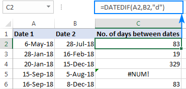
Track Recruitment Applications in Excel | ElyxAI
The article 'Track Recruitment Applications in Excel' by ElyxAI provides a great overview of these formulas in a recruitment context. Focus on the section explaining how to calculate the days since an application was received.
Scroll to the section titled 'Calculate days since application with DATEDIF'. It provides the exact formula and explains its purpose in a recruitment workflow.
Your Turn: Add the "Days in Pipeline" Column
- Open the
MasterTrackerfile you created in the previous lesson. - Go to the first empty column to the right of your table, and in the header row, type Days in Pipeline. Press Enter. Excel should automatically expand the table.
- In the first data cell of this new column, enter the
DATEDIFformula:
=DATEDIF([@[Application Date]], TODAY(), "d") - The formula should automatically fill down for all rows in the table. If any cells show a date instead of a number, select the column and change the format to Number in the Home tab.
2. Creating a "Current Status" Column
The Current Stage column is detailed, but for high-level reporting, managers often want to see a simplified status: Is the candidate Active, Hired, or Rejected? We can create a calculated column to automatically categorize each candidate.
To do this, we'll use the IFS function, which is a clean and modern way to handle multiple conditions. The logic is:
- If
Current Stageis "Hired", then the status is "Hired". - If
Current Stageis "Rejected", then the status is "Rejected". - Otherwise, the status is "Active".
Master the IF Formula in Excel (Beginner to Pro)
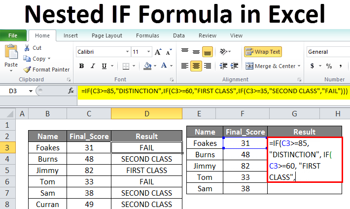
To understand how to handle multiple outcomes, watch this short segment from the 'Master the IF Formula in Excel' video by Kenji Explains. It introduces the IFS function, which we will use to create our Status column.
Watch the video from 02:01 to 03:51. Notice how the IFS function allows you to list pairs of conditions and results, making it much easier to read than deeply nested IF statements.
Your Turn: Add the "Status" Column
-
First, let's update our data to include all possible outcomes. In your
MasterTrackertable, change theCurrent Stagefor Olivia Chen toHiredand for Kenji Tanaka toRejected. This will give us data to test our formula against. -
Add a new column to your table named Status.
-
In the first cell of the
Statuscolumn, enter the followingIFSformula:=IFS([@[Current Stage]]="Hired", "Hired", [@[Current Stage]]="Rejected", "Rejected", TRUE, "Active")Let's break this down:
[@[Current Stage]]="Hired", "Hired": If the stage is "Hired", return "Hired".[@[Current Stage]]="Rejected", "Rejected": If the stage is "Rejected", return "Rejected".TRUE, "Active": This is the default case. If none of the previous conditions are met, the formula evaluatesTRUEand returns "Active". This is a clean way to handle the "else" condition.
Your Status column should now show the correct simplified status for every candidate.
3. Calculating "Time to Decision"
Now let's tackle a more advanced "time-in-stage" metric: Time to Decision. This KPI measures the number of days from when a candidate applied to when a final decision ("Hired" or "Rejected") was made. For candidates who are still "Active," this should remain blank.
Your Turn: Add "Time to Decision"
-
First, we need a date for when the decision was made. Add a new column to your table called Decision Date.
-
For the two candidates with a final status, enter a
Decision Date.- For Olivia Chen (Hired), enter
2024-10-28. - For Kenji Tanaka (Rejected), enter
2024-10-29. - Leave this column blank for all "Active" candidates.
- For Olivia Chen (Hired), enter
-
Now, add a final column named Time to Decision.
-
In the first cell, enter this formula:
=IF([@[Decision Date]]<>"", [@[Decision Date]]-[@[Application Date]], "")This formula checks if the
Decision Dateis not blank (<>"").- If it's not blank, it calculates the difference between the
Decision DateandApplication Date. - If it is blank, it returns an empty string (
""), keeping the cell clean for active candidates.
- If it's not blank, it calculates the difference between the
Ensure the Time to Decision column is formatted as a Number. You now have a precise measure of your hiring efficiency for completed applications.
4. Helper Columns for Easy Summarization
Our final step is to prepare the data for the next stage: creating summary reports with PivotTables. A powerful technique for this is to use "helper columns" that convert statuses into numbers (1 or 0). This makes it incredibly simple to sum up counts.
Recruitment Dashboard using Excel - - Excel Highway
The article 'Recruitment Dashboard using Excel' from Excel Highway mentions this exact technique. It uses simple IF statements to create 'counter' columns for different statuses.
Read the bullet point list under the heading 'Counting fields'. Notice the simple formulas used for 'Offer counter', 'Accepted counter', and 'Hired counter'. We will apply the same logic.
Your Turn: Add Counter Columns
Add the following three helper columns to your MasterTracker table, using the simple IF formulas provided.
- Hired Counter
- Formula:
=IF([@Status]="Hired", 1, 0)
- Formula:
- Rejected Counter
- Formula:
=IF([@Status]="Rejected", 1, 0)
- Formula:
- Active Counter
- Formula:
=IF([@Status]="Active", 1, 0)
- Formula:
When you create a PivotTable in our next lesson, you can simply drag the "Hired Counter" field into the Values area and select SUM to get an instant count of all hired candidates.
Conclusion
In this lesson, you significantly enhanced the MasterTracker. You moved beyond raw data entry and started creating valuable business intelligence.
Here are your key takeaways:
- You used
DATEDIFandTODAY()to calculate the Days in Pipeline, a key measure of recruitment velocity. - You used the
IFSfunction to create a simplified Status column (Active,Hired,Rejected), which is perfect for high-level reporting. - You calculated the Time to Decision, a critical efficiency metric, for completed applications.
- You added numerical Counter Columns that will make creating summary reports with PivotTables incredibly fast and easy.
Your data is no longer just a list of names; it's an analytical dataset, rich with metrics. In the next lesson, we will leverage these new columns to build a PivotTable summary that shows candidate counts by pipeline stage and recruiter, turning our detailed table into a powerful, interactive report.