Introduction
Welcome to the fourth lesson of your Recruitment Pipeline capstone project. In our last session, you did an excellent job of taking the raw MasterTracker data and summarizing it with a PivotTable. You now have a report that cleanly shows the number of candidates each recruiter is managing at every stage of the pipeline.
This lesson builds directly on that work to achieve our next learning outcome: to create a dashboard to visualize recruitment funnel metrics and recruiter performance.
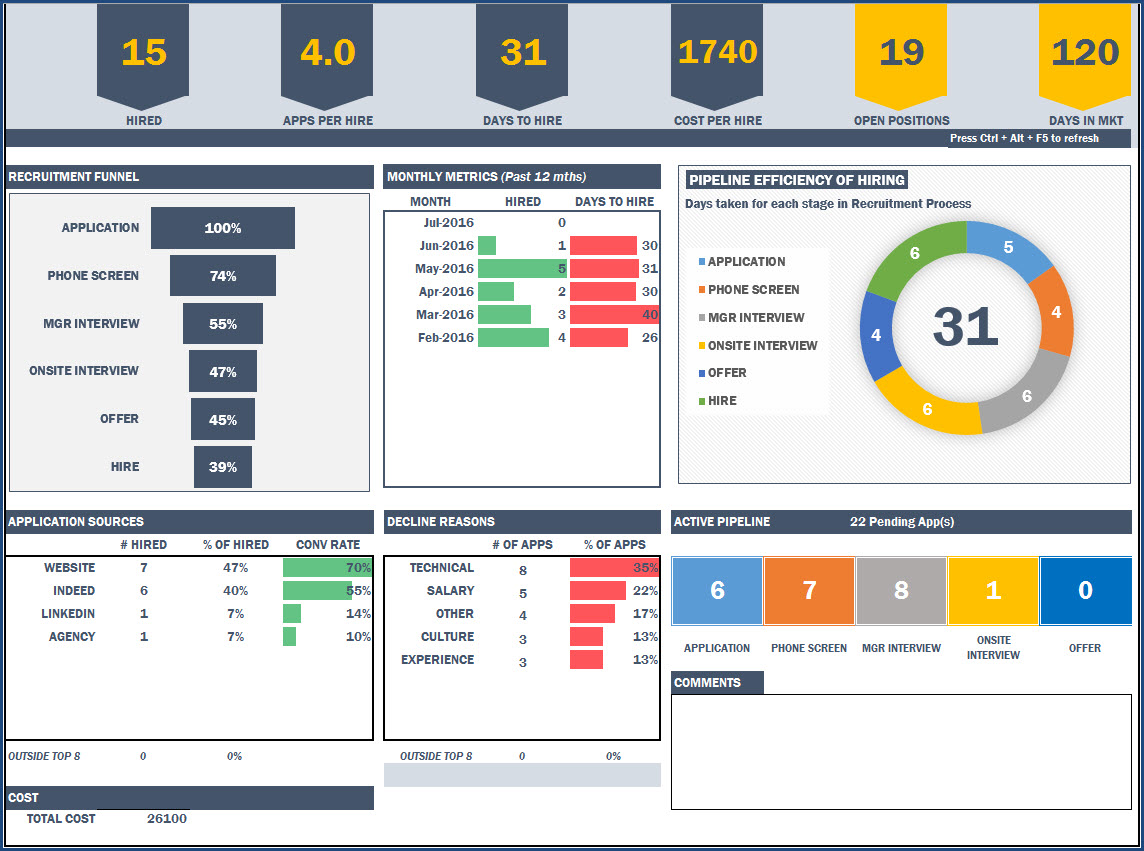
A dashboard is the most visible and impactful output for an MIS Executive. It's a single screen that uses charts and interactive filters to tell a story with data. Instead of just presenting a table of numbers, you will create a dynamic tool that allows managers to see the recruitment pipeline's health at a glance. We will transform your PivotTable summary into engaging visuals that answer key business questions instantly.
1. What is a Recruitment Dashboard?
Before we start building, it's useful to understand the purpose of a recruitment dashboard. It's a command center for hiring, providing a real-time, bird's-eye view of your most important hiring metrics.
HR Guide to Recruiting Dashboards
To get a clear picture of what a recruitment dashboard accomplishes and what key metrics it should include, read the first few sections of this article from Wellhub.
Please read the sections titled "What Is a Recruiting Dashboard, and Why Does it Matter?" and "Essential Recruiting Metrics & KPIs". Focus on how a dashboard moves beyond raw data to provide actionable insights.
As the article mentions, a good dashboard visualizes key metrics. Today, we'll focus on two core components:
- Recruiter Performance: How many active candidates is each recruiter handling?
- Recruitment Funnel: How efficiently are we moving candidates from application to hire?
2. Setting Up the Dashboard Canvas
Best practice in Excel is to keep your raw data, your calculations (like PivotTables), and your final dashboard on separate worksheets. This keeps your workbook organized and easy to maintain.
- Open your
MasterTrackerExcel file from the previous lesson. - Create a new worksheet and name it Dashboard. This will be your presentation layer.
- To give it a clean, professional look, go to the View tab and uncheck Gridlines. This removes the cell borders and makes the sheet look like a blank canvas.
- Optionally, you can add a title at the top, for instance in cell A1: "Recruitment Pipeline Dashboard".
3. Visualizing Recruiter Performance with a PivotChart
Let's start by visualizing the PivotTable you created in the last lesson. A PivotChart is a chart that is linked directly to a PivotTable, meaning it will update automatically when the PivotTable's data changes or is filtered.
The most efficient way to learn this is by watching a demonstration.
📊 How to Build Excel Interactive Dashboards
This video by Kevin Stratvert provides an excellent walkthrough of building an interactive dashboard. We will focus on the sections covering PivotCharts and arranging them on a dashboard sheet.
Please watch from 06:26 to 12:51. Pay close attention to these steps: How to insert a PivotChart from an existing PivotTable (06:36). How to clean up the chart by giving it a title and hiding the field buttons (07:30). How to cut and paste the chart onto the dashboard sheet (08:06). How to align multiple charts for a clean layout (12:15).
Your Turn: Create the Recruiter Performance Chart
Now, apply those steps to your own data.
- Go to the worksheet containing the PivotTable you built in the last lesson (the one with
Pipeline Stagein Rows andRecruiterin Columns). - Click anywhere inside your PivotTable.
- Go to the PivotTable Analyze tab on the ribbon and click PivotChart.
- In the Insert Chart dialog, choose a Stacked Column chart and click OK. A stacked column chart is great here because it shows each recruiter's total candidate load while also showing the breakdown by stage.
- Clean up the chart:
- Click on the chart title and change it to something meaningful, like "Active Candidates by Recruiter".
- Right-click on one of the grey "field buttons" on the chart (e.g., the one that says "Pipeline Stage") and select Hide All Field Buttons on Chart. This makes it look much cleaner.
- Move the chart:
- Select the chart.
- Press
Ctrl+Xto cut it. - Go to your Dashboard sheet.
- Press
Ctrl+Vto paste it.
.
- Position and resize the chart to fit nicely on the left side of your dashboard.
You now have your first dashboard component!
4. Building the Recruitment Funnel Chart
A funnel chart is a classic visualization for tracking recruitment. It shows how many candidates progress through each stage, making it easy to spot bottlenecks. While Excel has a built-in Funnel chart type, it's not easily connected to a PivotTable. We will use a more powerful and flexible technique: a customized stacked bar chart.
This involves creating a small helper table to calculate an "offset" that centers the bars, creating the funnel illusion.
How to Build a Recruitment Funnel Chart in Excel
This video from Indzara demonstrates the exact technique we will use. It's a bit clever, but the result is a professional and dynamic funnel chart.
Watch from 06:17 to 13:11. Don't worry about the COUNTIFS formulas at the beginning; we will use a PivotTable. Focus on understanding the logic behind: The cumulative count (06:28): Calculating how many candidates made it to or past each stage. The 'offsetter' calculation (08:42): This is the key trick. Understand that its purpose is to create an invisible spacer to center the visible bar. Adding the offsetter series to the chart and then hiding it (10:21) by setting its fill to 'No Fill'.
Your Turn: Create the Funnel Chart
Let's break this down into manageable steps.
Step 1: Create a New PivotTable for the Funnel
- Go back to your
MasterTrackerdata sheet and click anywhere in the table. - Insert a new PivotTable on a New Worksheet. Let's rename this new sheet to Calcs. This sheet will hold all our background calculations.
- Drag
Current Stageinto the Rows area. - Drag
Candidate IDinto the Values area and set it to Count. - Sort the stages in the correct funnel order (e.g., Screening, Interview, Offer). You can do this by manually dragging the row labels in the PivotTable.
Step 2: Build the Helper Table
On the same Calcs sheet, to the right of your new PivotTable, create a small table with four columns: Stage, Cumulative Count, Offsetter, and Actual Count.
- Stage: Manually type or copy the stage names from your PivotTable, in the correct funnel order.
- Actual Count: Use simple cell references to pull the counts from your PivotTable. For example, if your first stage count is in cell
B4, the formula is just=B4. - Cumulative Count: This is the count of candidates who reached the current stage or any subsequent stage.
- In the cell for your last stage (e.g.,
Offer), the formula will be the same as its actual count. - For the stage above it (
Interview), the formula will be:(Interview's Actual Count) + (Offer's Cumulative Count). - Continue this pattern all the way to the top. The top stage (
Screening) should have a cumulative count equal to the total number of candidates.
- In the cell for your last stage (e.g.,
- Offsetter: This calculates the size of the invisible bar needed to center the real bar. The formula for each row is:
(Cumulative Count of the TOP stage - This stage's Cumulative Count) / 2. Make sure you use an absolute reference ($) for the top stage's cumulative count.
Step 3: Create and Format the Chart
- Select the
Stage,Cumulative Count, andOffsettercolumns in your helper table. - Go to Insert > Chart and choose a 2D Stacked Bar chart.
- Right-click the vertical axis (the stage names) and select Format Axis. In the Axis Options, check the box for Categories in reverse order. This puts the 'Screening' stage at the top.
- Click on the bars representing the Offsetter series. In the Format tab, set the Shape Fill to No Fill. They are now invisible spacers.
- Add Data Labels to the visible bars (the
Cumulative Countseries). Format them to be centered. - Clean up the chart: Give it a title ("Recruitment Funnel"), remove the legend, and remove the horizontal axis at the bottom.
- Cut (
Ctrl+X) the chart and paste (Ctrl+V) it onto your Dashboard sheet. Position it next to your first chart.
5. Making the Dashboard Interactive with Slicers
Now for the final and most powerful step: making the dashboard interactive. Slicers are user-friendly buttons that filter your PivotTables (and therefore your PivotCharts).
📊 How to Build Excel Interactive Dashboards
Let's return to the Kevin Stratvert video to see how to add slicers and, most importantly, connect them to all of our charts.
Watch from 12:51 to 16:05. The most critical part is at 14:55, where he demonstrates how to connect a single slicer to multiple PivotTables using 'Report Connections'. This is what makes your entire dashboard update at once.
Your Turn: Add and Connect Slicers
- Click on your Recruiter Performance chart on the dashboard.
- Go to the PivotChart Analyze tab and click Insert Slicer.
- In the dialog box, choose the fields you want to filter by. Let's pick
RecruiterandJob Title. Click OK. - Two slicer boxes will appear. Position them neatly on your dashboard, perhaps on the right side or along the top.
- This is the most important step. By default, these slicers only control the PivotTable they were created from. You must connect them to your funnel chart's PivotTable as well.
- Right-click on the Recruiter slicer.
- Select Report Connections....
- In the dialog box, you'll see a list of all PivotTables in your workbook. Check the box next to the PivotTable you created for the funnel chart (it might be named
PivotTable2). Click OK. - Repeat this process for the Job Title slicer.
Now, test it! Click on a recruiter's name in the slicer. Both the Recruiter Performance chart and the Funnel chart should update to show data for only that recruiter. You have just built a fully interactive dashboard.
Conclusion
Fantastic work today! You have successfully moved from a static summary table to a dynamic, visual, and interactive dashboard. This is a huge step in your journey to becoming an MIS Executive, as it demonstrates your ability to not just process data, but to present it in a way that is insightful and easy for stakeholders to understand.
Here are your key takeaways:
- A dashboard is a single-sheet view that visualizes key metrics using charts and interactive filters.
- PivotCharts are a quick way to create dynamic charts directly from your PivotTable summaries.
- Advanced visualizations like a recruitment funnel can be created in Excel using clever techniques like a stacked bar chart with an invisible "offsetter" series.
- Slicers are user-friendly buttons that filter dashboard data.
- The Report Connections feature is crucial for linking a single slicer to multiple PivotTables, ensuring your entire dashboard updates in sync.
In our final lesson, you will learn how to put all these pieces together to assemble a professional weekly MIS report with charts, summary tables, and analytical commentary. The dashboard you built today will be the central component of that final deliverable.