Structured References for Dynamic Formulas

1. The "Why": Structured References vs. Traditional Ranges

Imagine you're summing a column of sales data. With a traditional range, your formula would be =SUM(F3:F6). If you add a new sale in row 7, you must remember to manually update the formula to =SUM(F3:F7). Forgetting to do this is a common source of major errors in MIS reports.

Now, look at the difference with an Excel Table.

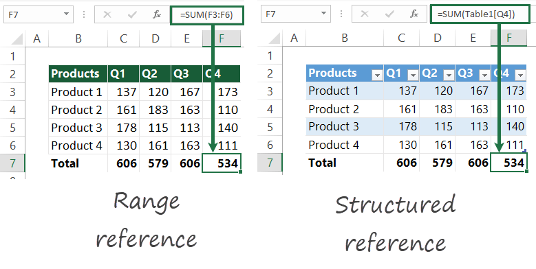
The formula on the right, =SUM(Table1[Q4]), uses a structured reference. It's easier to read because it tells you exactly what you're summing: the 'Q4' column from 'Table1'. More importantly, because it's linked to a Table, this formula will automatically include any new data added to that column. This dynamic nature is what makes Tables and structured references so essential for reliable reporting.

2. Writing Formulas with Structured References

There are two main places you'll use structured references: inside the table to create new calculated columns, and outside the table to create summary reports.

Inside the Table: Calculated Columns

Let's say you want to add a new column to your table that calculates a value for each row. For example, multiplying "Quantity" by "Unit Price" to get "Total Cost".

The formula shown, =[@Quantity]*[@[Unit Price]], uses a special syntax.

• The square brackets [] tell Excel you are referring to a table column.
• The @ symbol is shorthand for "this row".

So, [@Quantity] means "get the value from the 'Quantity' column in this current row".

When you enter this formula in the first cell of the new column and press Enter, the Table automatically copies it down to all the other rows. This is called a calculated column, and it ensures the same formula is applied consistently throughout your data.

To see this in action, let's watch a short segment of a video.

Outside the Table: Summary Formulas

When you write a formula outside the table to summarize data (like a SUM or COUNT), you use a slightly different format: TableName[ColumnName].

This is called a fully qualified reference because you specify both the table name and the column name. This tells Excel exactly where to find the data, no matter where in the workbook you write the formula.

For a great practical demonstration of using structured references in summary formulas, please review the following guide.

3. The Anatomy of a Structured Reference

Structured references have a specific syntax that lets you refer to different parts of a table precisely. These parts are called specifiers.

The video below gives an excellent breakdown of the most common specifiers. We'll watch a few key clips to understand them.

Here is a summary table of the key components you'll use most often. Let's assume your table is named Tracker.

Don't worry about memorizing all of these right now. The most important ones to master first are Tracker[Column] and [@Column]. Excel's Formula AutoComplete will help you with the rest as you type.

4. Hands-On Practice

Let's apply these concepts to the Recruitment_Tracker table you created in the last lesson. If you don't have it open, re-create it quickly with the following data, convert it to a Table (Ctrl+T), and name it Recruitment_Tracker.

Candidate ID,Full Name,Position,Stage,Applied Date,Source
C-001,Amit Kumar,Cyber Analyst,Interview,2024-05-01,LinkedIn
C-002,Priya Sharma,Jr. Project Coordinator,Offer,2024-05-02,Naukri
C-003,Rahul Verma,MIS Executive,Screening,2024-05-03,LinkedIn
C-004,Sneha Patil,Cyber Analyst,Hired,2024-05-03,Internal
C-005,Neha Singh,MIS Executive,Interview,2024-05-04,Naukri

Task 1: Add a Calculated Column

As a recruitment coordinator, you often need to know how long a candidate has been in the pipeline. Let's calculate the number of days since they applied.

1. Go to cell G1 (the first empty column next to your table) and type the header Days in Pipeline. Press Enter. The table will automatically expand.
2. In cell G2, type the following formula: =TODAY()-[@[Applied Date]]
3. Press Enter.
   • TODAY() is an Excel function that returns the current date.
   • [@[Applied Date]] uses the current row specifier (@) to get the application date for that specific row.
   • Notice how the formula automatically fills down the entire column. You now have a dynamic calculation of aging for each candidate.

Task 2: Create an External Summary Area

Now, let's create a small summary dashboard to the right of your table. This is a typical task for an MIS report.

1. In cell I2, type the label Total Candidates.

2. In cell J2, enter the formula: =COUNTA(Recruitment_Tracker[Candidate ID])

   • This formula counts all non-blank cells in the Candidate ID column of the Recruitment_Tracker table.

3. In cell I3, type the label Candidates in Interview.

4. In cell J3, enter the formula: =COUNTIF(Recruitment_Tracker[Stage],"Interview")

   • This formula counts how many times the word "Interview" appears in the Stage column.

Now for the magic. Go to row 8 and add a new candidate. Watch how the Total Candidates count in cell J2 updates instantly. This is the power of building reports on Tables with structured references.

Key Takeaways

• Structured references replace cell addresses (D2:D10) with readable names (TableName[ColumnName]).
• They make formulas dynamic, automatically updating when your table data changes.
• Use [@ColumnName] to perform row-by-row calculations inside a table (calculated columns).
• Use TableName[ColumnName] to summarize data outside the table.
• Mastering this syntax is crucial for building the robust, automated trackers and MIS reports that employers value.

Next Lesson

Excellent work! You've now mastered the two core components of structuring data in Excel: creating Tables and using structured references to work with them.

In the next lesson, we will explore a related concept: defining and using Named Ranges. While Tables are for structured, row-by-row data, Named Ranges are perfect for single cells or fixed ranges that hold important constants, like a tax rate, a target value, or a list of regions. Using them will make your formulas even clearer and easier to manage.