Unlocking Dynamic Features with Excel Tables

1. From a Static Range to a Dynamic Table

So far, the data we've worked with has been in a "range"—a simple grid of cells. A range is static. If you build a chart or a summary formula based on a range like A1:E50, it will not automatically update if you add a new row of data at row 51. You would have to manually update all your formulas and chart sources. This is inefficient and a major source of errors in MIS reporting.

An Excel Table is a special container that tells Excel your data belongs together. By converting a range into a Table, you unlock powerful dynamic features that automate many of these manual tasks.

To get a quick overview of why this is so important, please read the first section of the following article.

The key takeaway is that Tables turn your static data into a dynamic object that Excel can manage intelligently.

2. How to Create an Excel Table

Creating a Table is simple. The main prerequisite is that your data should be in a clean, tabular format with a unique header for each column, which is something you've already practiced.

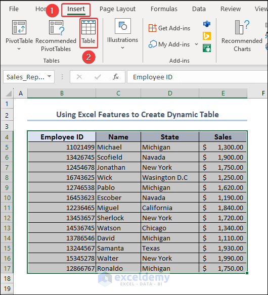
Let's watch a short video that demonstrates the most common ways to convert a data range into a Table.

The keyboard shortcut Ctrl + T is the method most professionals use because it's fast and efficient. Try to make it a habit.

Once you create a Table, a new Table Design tab appears on the ribbon whenever you click inside the Table. This is your command center for managing the Table.

3. The Power of "Dynamic Features"

Now for the most important part: understanding what makes a Table "dynamic." This is the core reason we use them. The following video provides an excellent demonstration of these features.

To summarize the key dynamic features:

• Automatic Range Expansion: When you type or paste data in the row immediately below the Table, or the column immediately to its right, the Table automatically expands to include it. All formulas, charts, and PivotTables based on this Table will update instantly. This is the cornerstone of automated reporting.
• Easy, Consistent Formatting: You can apply or change professional formatting styles with a single click from the Table Design tab. The formatting also automatically extends to new rows.
• Intelligent Formula Fill-Down: In later lessons, when we write formulas in a Table column, they will automatically fill down to every row, ensuring consistency.

Hands-On Practice

Let's apply what you've learned. Your experience in recruitment involved tracking candidates, so we'll use a simplified version of that data.

1. Open a new Excel workbook.
2. Copy the data below and paste it into cell A1.

Candidate ID,Full Name,Position,Stage,Applied Date
C-001,Amit Kumar,Cyber Analyst,Interview,2024-05-01
C-002,Priya Sharma,Jr. Project Coordinator,Offer,2024-05-02
C-003,Rahul Verma,MIS Executive,Screening,2024-05-03
C-004,Sneha Patil,Cyber Analyst,Hired,2024-05-03

Now, let's turn this into a dynamic tracker.

Task 1: Convert to an Excel Table

• Click anywhere inside the data (e.g., cell B2).
• Press Ctrl + T.
• In the "Create Table" dialog box, ensure the range is correct (=$A$1:$E$5) and the "My table has headers" box is checked.
• Click OK. Your data is now a formatted Table with filter buttons.

Task 2: Name Your Table

• Click anywhere inside your new Table.
• Go to the Table Design tab that appears on the ribbon.
• In the "Table Name" box on the far left, replace the default name (like Table1) with a descriptive name: Recruitment_Tracker. Press Enter. (Note: Table names cannot contain spaces).

Task 3: Witness the Dynamic Expansion

• Go to cell A6, which is the first cell directly below your Table.
• Type in the next Candidate ID: C-005. Press Enter.
• Notice how the Table automatically expands to include this new row, complete with the formatting. You can now fill in the rest of the data for this candidate: Neha Singh, MIS Executive, Interview, 2024-05-04.
• Now, go to cell F1, the first cell to the right of your Table. Type the header Source and press Enter.
• Again, the Table automatically expands to include this new column. You can now fill in the source for each candidate (e.g., LinkedIn, Naukri).

You've just experienced the primary benefit of Excel Tables. Any report or chart you build on Recruitment_Tracker will now automatically include new candidates and new data fields without any manual updates.

Summary of Key Takeaways

• A standard Excel range is static, while an Excel Table is a dynamic container for your data.
• To create a Table, click in your data and press Ctrl + T.
• Always give your tables a meaningful name via the Table Design tab.
• The key dynamic feature of a Table is its ability to automatically expand to include new rows and columns, which is essential for building automated reports.

Next Lesson

Fantastic! You now know how to properly structure data in Excel. This is a massive step forward and a skill that many Excel users overlook.

In our next lesson, we will leverage this new structure to write cleaner, more powerful formulas. You will learn how to use structured references to refer to Table data by name (e.g., Recruitment_Tracker[Stage]) instead of by cell addresses (e.g., D2:D6). This makes formulas much easier to read, write, and maintain.