Retrieving Data with VLOOKUP

1. What is VLOOKUP and How Does It Work?

VLOOKUP stands for Vertical Lookup. Its job is to search for a specific value (like an Employee ID or an Incident Number) in the first column of a table and return a corresponding piece of information from a different column in that same row.

Imagine you have two lists:

1. A Daily Incident Log: Contains Incident ID, Date, and Assigned Analyst ID.
2. An Analyst Master List: Contains Analyst ID, Full Name, and Team.

Your task is to add the Full Name of the analyst to your Daily Incident Log. VLOOKUP is the perfect tool for this. It will look up the Analyst ID from your incident log in the master list and return the Full Name.

The syntax for the function is:
=VLOOKUP(lookup_value, table_array, col_index_num, [range_lookup])

This might look complex, but each part has a simple job:

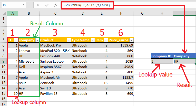
1. lookup_value: The piece of data you already have. In our example, this would be the Analyst ID in your incident log.
2. table_array: The table where you want to search for your data. This would be your Analyst Master List. A critical rule is that the lookup_value must be in the first column of this table.
3. col_index_num: The number of the column in the table_array that contains the information you want to retrieve. You count from the left, so the first column is 1, the second is 2, and so on.
4. [range_lookup]: This tells Excel whether you want an exact match (FALSE) or an approximate match (TRUE). For 99% of MIS work, you will use FALSE to ensure your data is accurate.

2. Building Your First VLOOKUP Formula

Theory is one thing, but seeing it in action makes it click. The best way to learn VLOOKUP is to build one step-by-step.

As you saw in the video, constructing the formula is a logical process of telling Excel:

1. What to look for.
2. Where to look for it.
3. Which column's information to bring back.
4. To find an exact match.

3. Avoiding the Two Most Common VLOOKUP Mistakes

VLOOKUP is powerful, but it's easy to make mistakes that lead to errors or, even worse, incorrect results. Let's tackle the two biggest ones head-on.

Mistake #1: Forgetting FALSE for an Exact Match

The [range_lookup] argument is optional, and if you leave it blank, Excel defaults to TRUE (approximate match). This can be disastrous for business data. It might "find" a close match and return the wrong information, which compromises your entire report.

For MIS and data tracking purposes, you should almost always specify FALSE to ensure you are only getting data for the exact ID or code you are looking up.

Mistake #2: The table_array Shifts When You Copy the Formula

After you write a VLOOKUP in one cell, you'll want to drag it down to apply it to the whole column. Often, this results in #N/A errors for the rows below. This happens because Excel's default cell references are relative. When you drag the formula down, the reference to your table_array also moves down, and it no longer looks at the complete master list.

There are two ways to solve this:

1. The Good Way: Absolute References ($)
   You can "lock" the table_array reference by adding dollar signs ($) to the cell addresses (e.g., $A$2:$C$50). The easiest way to do this is by highlighting the range in your formula and pressing the F4 key.

2. The Better Way: Excel Tables
   As we covered in a previous module, converting your data range into a structured Excel Table (Insert > Table) gives it a name. When you use this table in your formula, the reference is automatically locked and will even expand if you add new data to it. This is the most robust method for MIS work.

Kevin Stratvert's video explains both of these solutions clearly.

4. VLOOKUP in a Real-World Context: A Recruitment Tracker

Let's connect this to your experience in recruitment. A common task is to create a small dashboard where you can select a candidate's ID and instantly see their name, status, and other details. This is a perfect use case for VLOOKUP.

You would have two sheets:

• A Dashboard sheet with a cell to input the Applicant ID.
• An Applicants Info sheet with a master table of all candidates.

The VLOOKUP formula on the dashboard would look up the ID you entered and pull the relevant details from the master table.

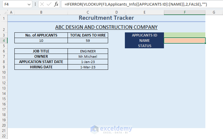
To see how this is built, you can review the following guide. It aligns perfectly with your goal of building trackers.

Key Takeaways

• VLOOKUP searches for a value in the first column of a table and returns a corresponding value from a column to the right.
• The syntax is =VLOOKUP(lookup_value, table_array, col_index_num, [range_lookup]).
• For accurate business reporting, always use FALSE (or 0) as the fourth argument for an exact match.
• When copying a VLOOKUP formula down, you must "lock" your table_array using absolute references ($) or, preferably, by referencing a named Excel Table.
• A key limitation: VLOOKUP cannot look to the left. The value you want to return must be in a column to the right of the lookup column.

Next Lesson

You've now learned the most famous lookup function in Excel. It's a workhorse for data consolidation. However, its limitation of only looking to the right and its reliance on column numbers can be cumbersome.

In the next lesson, we will explore XLOOKUP. This is the modern, more powerful, and more flexible successor to VLOOKUP. You'll see how it overcomes VLOOKUP's main weaknesses, making your lookup tasks even easier and more robust.