Welcome back! In our previous lesson, you mastered VLOOKUP, the classic tool for pulling data from one table into another. You learned its syntax, how to use it for exact matches, and how to avoid common errors by locking cell references.
However, you also discovered its main limitation: VLOOKUP can only search in the first column of a table and return a value from a column to its right. This can be restrictive, sometimes forcing you to rearrange your data.
Today, we'll learn the modern and more powerful solution that addresses all of VLOOKUP's shortcomings. We will focus on this lesson's outcome: Use XLOOKUP to perform flexible lookups (left, right, top, or bottom).
XLOOKUP is the successor to both VLOOKUP and HLOOKUP. It's more intuitive, more flexible, and safer to use. By the end of this lesson, you will understand why XLOOKUP is the new standard for lookups in Excel and be able to use it to retrieve data regardless of how your tables are structured.
1. Understanding the Core of XLOOKUP
At its heart, XLOOKUP does the same job as VLOOKUP: it finds a value in one list and returns a corresponding value from another. The key difference is its simpler and more logical syntax.
The basic syntax for XLOOKUP is:=XLOOKUP(lookup_value, lookup_array, return_array)
Let's break this down:
lookup_value: The value you want to search for (e.g., an Incident ID, a candidate's name).lookup_array: The column or row where you want to search for thelookup_value.return_array: The column or row that contains the value you want to get back.
Notice two immediate improvements over VLOOKUP:
- You select the lookup and return columns separately. There is no more counting columns (
col_index_num). - The lookup column does not have to be the first one in a table array.
Let's watch a quick tutorial to see this basic structure in action.
How to Use XLOOKUP in Excel – Step-by-Step Tutorial for Beginners
This video from Kevin Stratvert provides a very clear introduction to the XLOOKUP function. It will help you get comfortable with the three main arguments.
Watch from the beginning to 02:21. Pay attention to how he defines the lookup_value, lookup_array, and return_array. You'll notice it feels more direct than setting up a VLOOKUP.
A Quick Reminder on Copying Formulas
Just like with VLOOKUP, when you copy an XLOOKUP formula down a column, you need to "lock" your arrays so they don't shift. The F4 key is your best friend here for adding absolute references ($).
How to Use XLOOKUP in Excel – Step-by-Step Tutorial for Beginners
Let's revisit Kevin's video to see how to properly lock the ranges before copying the formula.
Watch from 04:50 to 06:17. He demonstrates exactly why formulas break when copied and how to fix it by applying absolute references to the lookup_array and return_array.
2. The Power of Flexibility: Looking in Any Direction
This is where XLOOKUP truly shines and directly addresses our learning goal. It doesn't care where your return column is relative to your lookup column.
Looking to the Left
In your past work with incident response, you might have had a master employee list where the Employee Name was in column A and their Employee ID was in column B. With VLOOKUP, you couldn't look up an employee's name using their ID without rearranging the columns. XLOOKUP solves this effortlessly.

Looking Horizontally (Up or Down)
XLOOKUP also replaces HLOOKUP (Horizontal Lookup). You can use the exact same formula structure to look up a value in a row and return a corresponding value from another row above or below it. This is useful for financial reports or any data organized by time periods across columns.
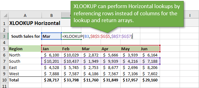
To see these flexible lookups demonstrated, let's turn to a more comprehensive tutorial.
XLOOKUP Complete Tutorial in Excel (+ Hidden Tricks)
The 'XLOOKUP Complete Tutorial' from MyOnlineTrainingHub covers many advanced uses. We'll focus on the sections for left and horizontal lookups.
Please watch these two specific segments: Horizontal Lookup (HLOOKUP replacement): Watch from 02:47 to 03:20. Left Lookup (VLOOKUP's biggest weakness): Watch from 16:18 to 17:12. Notice how the logic of the formula doesn't change at all.
3. Exploring XLOOKUP's Optional Arguments
XLOOKUP has three optional arguments that add even more power and safety. While you will mostly use the first three, being aware of these is crucial for an MIS role.
The full syntax is:=XLOOKUP(lookup_value, lookup_array, return_array, [if_not_found], [match_mode], [search_mode])
[if_not_found]: What to show if no match is found. Instead of getting an#N/Aerror and wrapping your formula inIFERROR(which we will cover soon), you can just tellXLOOKUPwhat to display, for example, "Not Found" or0.[match_mode]: This controls the type of match.0- Exact match (This is the default, makingXLOOKUPmuch safer thanVLOOKUP!).-1- Exact match, or the next smaller item (useful for tax brackets or commission tiers).1- Exact match, or the next larger item.
[search_mode]: This controls the search direction.1- Search from first-to-last (the default).-1- Search from last-to-first. This is incredibly useful for finding the most recent entry for a specific ID, like the latest status of an incident or a candidate in a log.
This article provides a great summary of the syntax if you want a quick reference.
Excel XLOOKUP function - syntax and uses
The article 'Excel XLOOKUP Function' from Ablebits.com has a very clear breakdown of the function's syntax and arguments. It's a useful resource to bookmark.
Review the section 'Excel XLOOKUP function - syntax and uses'. It provides a concise explanation of all six arguments.
4. Hands-On Practice: Incident & Recruitment Data
Let's apply what you've learned. Imagine you have two tables in Excel.
Table 1: Incidents_Log
| Incident ID | Date | Category | Assigned_To_ID |
|---|---|---|---|
| INC-001 | 01-Feb | Phishing | EMP-105 |
| INC-002 | 01-Feb | Malware | EMP-102 |
| INC-003 | 02-Feb | Phishing | EMP-105 |
Table 2: Analyst_Roster (in a different location, maybe on another sheet)
| Analyst Name | Team | Employee_ID |
|---|---|---|
| Alice Johnson | Tier 1 | EMP-102 |
| Bob Williams | Tier 2 | EMP-105 |
| Charlie Brown | Tier 1 | EMP-108 |
Your Tasks:
-
Perform a Left Lookup: In the
Incidents_Logtable, add a new column calledAnalyst Name. Write anXLOOKUPformula to pull the correct analyst's name from theAnalyst_Rostertable using theAssigned_To_ID.- Hint: Your
lookup_valueis the ID in the incidents table. Yourlookup_arrayis the ID column in the roster. Yourreturn_arrayis the name column in the roster.
- Hint: Your
-
Use
if_not_found: What if you had an incident assigned toEMP-109, who is not in the roster? Modify your formula to return the text "Unassigned" instead of an#N/Aerror.
Click here to see the solution formulas
For Task 1: Assuming your Incidents_Log is in A1:D4 and Analyst_Roster is in F1:H4, the formula in cell E2 of the Incidents_Log would be:=XLOOKUP(D2, $H$2:$H$4, $F$2:$F$4)
(Remember to use F4 to lock the arrays before dragging the formula down!)
For Task 2: The modified formula would be:=XLOOKUP(D2, $H$2:$H$4, $F$2:$F$4, "Unassigned")
Key Takeaways
XLOOKUPis the modern, flexible replacement for bothVLOOKUPandHLOOKUP.- Its core syntax
=XLOOKUP(lookup_value, lookup_array, return_array)is more intuitive and robust. - Its key advantage is the ability to look in any direction: left, right, up, or down.
- It defaults to an exact match, making it safer for data integrity.
- It has built-in error handling (
if_not_found) and can search in reverse order (search_mode), which are powerful features for MIS reporting.
Next Lesson
You've now added the most powerful lookup function to your toolkit. While XLOOKUP can handle almost any lookup scenario you'll encounter, it's still valuable to understand the classic "power user" alternative that preceded it: INDEX and MATCH. In the next lesson, we will explore how to combine these two functions to perform robust lookups, which is a skill you will frequently see in more complex, older spreadsheets.