Hello! Welcome to the third lesson in our module on core formulas for conditional logic.
In our last lesson, we focused on the IF function to categorize data based on business rules. You learned to build simple and nested IF statements to label your data—for example, marking an incident as "High Priority" or a sales figure as "On Target."
Today, we'll put those categories to work. This lesson addresses the learning outcome: Use COUNTIFS and SUMIFS to aggregate data based on multiple criteria. These two functions are the engine of almost every summary report and dashboard you will build as an MIS Executive. They allow you to move from a long list of raw data to a concise summary of key metrics.
We'll cover:
- The
SUMIFSfunction, to sum values that meet several conditions. - The
COUNTIFSfunction, to count rows that satisfy multiple criteria. - How to use comparison operators (like
>,<) and wildcards (*) to create flexible and powerful summaries. - A powerful technique for summarizing data based on a list of items.
This is a critical skill for creating the reports you'll be responsible for in an MIS role, such as summarizing incident data or tracking recruitment pipelines.
1. SUMIFS: Summing Values Based on Multiple Conditions
Imagine you have a large dataset of sales transactions, incidents, or candidate applications. You won't be presenting this raw data to management. Instead, you'll be asked for summaries like, "What were the total sales for 'Product A' in the 'North' region?" or "What is the total data volume breached in 'High' priority incidents caused by 'Phishing'?"
This is where SUMIFS is essential. It lets you sum a column of numbers, but only for the rows that meet all the conditions you specify.
The syntax is:=SUMIFS(sum_range, criteria_range1, criteria1, criteria_range2, criteria2, ...)
sum_range: The range of cells you want to add up (e.g., the 'Sales Amount' column).criteria_range1: The range where you'll look for your first condition (e.g., the 'Region' column).criteria1: The condition you're looking for (e.g., "North").- You can then add more pairs of
criteria_rangeandcriteria.
Notice that with SUMIFS, the range you are summing comes first. This is a key difference from its simpler predecessor, SUMIF. It's recommended to always use the SUMIFS version, even for a single condition, to maintain consistency.
The following video provides a clear, step-by-step walkthrough of the SUMIFS function.
How to Use SUMIFS, COUNTIFS and AVERAGEIFS in Excel (Multiple Criteria)
This video from Leila Gharani explains the syntax of SUMIFS and provides excellent, easy-to-follow examples. Pay close attention to the order of the arguments in the formula.
Watch from 03:18 to 06:02. The first part demonstrates a SUMIFS with two criteria, and the second part extends it to three, showing how simple it is to add more conditions.
2. COUNTIFS: Counting Rows with Multiple Conditions
While SUMIFS adds up values, COUNTIFS simply counts the number of rows that meet your criteria. This is perfect for answering questions like, "How many incidents are currently 'Open' and assigned to 'Team A'?" or "How many candidates from 'LinkedIn' have reached the 'Interview' stage?"
The syntax is very similar to SUMIFS, but without the sum_range because we are just counting rows:
=COUNTIFS(criteria_range1, criteria1, criteria_range2, criteria2, ...)
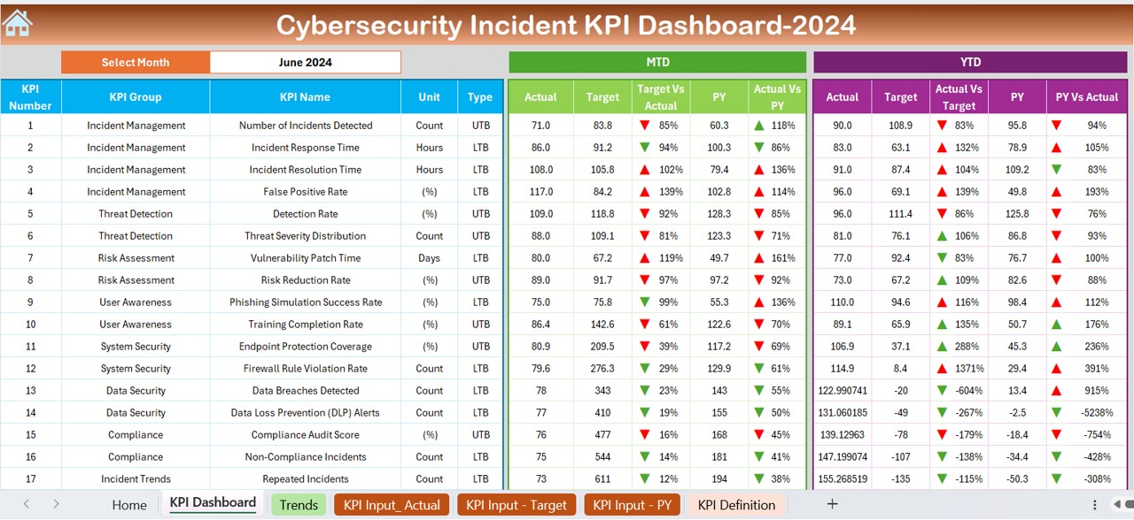
Let's look at a practical example from your background. The dashboard below tracks cybersecurity KPIs. A metric like "Incidents - MTD" for "Phishing" would be calculated using COUNTIFS.
Let's return to the video to see how COUNTIFS works.
How to Use SUMIFS, COUNTIFS and AVERAGEIFS in Excel (Multiple Criteria)
The same video also covers the COUNTIFS function. Notice how the structure is simpler because there is no 'sum range' to specify.
Watch from 10:20 to 11:08. The instructor demonstrates how to count occurrences based on multiple criteria, building on the same dataset.
3. Using Comparison Operators and Wildcards
Your criteria won't always be a simple text match. Often, you'll need to sum or count based on more flexible conditions.
-
Comparison Operators: You can use operators like
>,<,>=,<=, and<>(not equal to) for numerical or date-based criteria. For example, counting incidents with a data loss>100GB. Crucially, the operator and value must be enclosed in double quotes, like">100". -
Wildcards: The asterisk (
*) is a wildcard character that represents any sequence of characters. This is extremely useful for partial text matches. For example,"*Phishing*"would match "Phishing", "Spear Phishing", and "Phishing Attempt".
The next segment of the video demonstrates both of these powerful techniques.
How to Use SUMIFS, COUNTIFS and AVERAGEIFS in Excel (Multiple Criteria)
This part of the video explains how to incorporate comparison operators and wildcards into your SUMIFS formula. The syntax for this is very important to get right.
Watch from 06:02 to 09:07. Pay close attention to how the > operator is enclosed in quotes. Also, note how you can combine the operator with a cell reference using the & symbol, which is a common practice in MIS reports.
4. Practical Application and Best Practices
Now let's combine these concepts and add a few best practices that are essential for any MIS role.
Best Practice 1: Use Excel Tables
In a previous module, you learned how to create Excel Tables. When building summary reports, using a Table for your source data is a non-negotiable best practice. When you add new data to the bottom of your table, any SUMIFS or COUNTIFS formulas that reference it will automatically include the new rows. This prevents errors and saves you from manually updating your formula ranges.
How to Use SUMIFS, COUNTIFS and AVERAGEIFS in Excel (Multiple Criteria)
This final clip from the video demonstrates the power of using Excel Tables with your summary formulas. This is a crucial technique for creating dynamic, low-maintenance reports.
Watch from 11:08 to 12:20. See how adding a new row to the data range doesn't update the formula, but adding it to an Excel Table does.
Best Practice 2: Summarizing Multiple Items (OR Logic)
What if you need to sum sales for the "North" AND "East" regions combined? You could write two SUMIFS formulas and add them together. However, a more elegant way is to use an array constant ({}) inside your formula. This is a very common requirement in MIS reporting.
SUMIF, SUMIFS, COUNTIF and COUNTIFS For Multiple Values of Interest At Once
This article from olafusimichael.com explains an advanced but incredibly useful technique for using SUMIFS and COUNTIFS with multiple values for a single criterion.
Read the section titled 'Now to the very interesting parts.'. Focus on the formula for summing sales for multiple pizza types. Notice how the list of items is enclosed in curly braces {"Meatzaa","Hot Veggie",...} and the whole formula is wrapped in a SUM() function.
The formula structure is =SUM(SUMIFS(sum_range, criteria_range, {"Value1", "Value2", "Value3"})). This technique is a significant time-saver.
Hands-on Practice
Let's apply this. Consider this data from a recruitment tracker. Your task is to calculate two KPIs for a summary report.
| Candidate ID | Source | Stage | Role |
|---|---|---|---|
| C-201 | Interview | Analyst | |
| C-202 | Referral | Hired | Analyst |
| C-203 | Screen | Manager | |
| C-204 | Indeed | Screen | Analyst |
| C-205 | Hired | Analyst |
- KPI 1: Count the number of candidates who came from 'LinkedIn' and are currently past the 'Screen' stage (i.e., their stage is not "Screen").
- KPI 2: Count the total number of candidates for the 'Analyst' role that came from either 'LinkedIn' or 'Indeed'.
Think about how you would structure the COUNTIFS formulas.
Solutions:
-
KPI 1:
=COUNTIFS(B:B, "LinkedIn", C:C, "<>Screen")B:Bis the 'Source' column.C:Cis the 'Stage' column. We use the "not equal to" operator<>to exclude candidates at the "Screen" stage.
-
KPI 2:
=SUM(COUNTIFS(D:D, "Analyst", B:B, {"LinkedIn", "Indeed"}))D:Dis the 'Role' column.- We use the array
{"LinkedIn", "Indeed"}to count candidates from both sources who are also applying for the 'Analyst' role. The outerSUMadds the results together.
Key Takeaways
SUMIFSandCOUNTIFSare essential tools for aggregating data based on multiple, simultaneous conditions.- The syntax requires pairs of
criteria_rangeandcriteria. ForSUMIFS, thesum_rangeis the very first argument. - Use quotes for text criteria and for comparison operators (e.g.,
">500"). - The
*wildcard is powerful for matching partial text. - Always use Excel Tables for your source data to ensure your summary formulas update automatically as new data is added.
- To sum or count based on a list of OR conditions (e.g., "North" or "South"), use the
=SUM(SUMIFS(...{"item1", "item2"}))pattern.
Next Lesson
You've now mastered the core functions for conditional logic and summarization. You can categorize data with IF and then aggregate it into meaningful totals with SUMIFS and COUNTIFS.
In the next module, we will explore another fundamental pillar of data analysis in Excel: Lookup Formulas. We will start with using VLOOKUP to retrieve data from a vertical table. This skill is crucial when you need to combine or enrich your data, for example, by pulling a candidate's contact information from a master list into your daily recruitment tracker.